Heart¶

模型训练命令模型评估命令

正问题：受力分析求解逆问题：参数逆推求解

# linux
wget -c https://paddle-org.bj.bcebos.com/paddlescience/datasets/heart/heart_dataset.tar
# windows
# curl https://paddle-org.bj.bcebos.com/paddlescience/datasets/heart/heart_dataset.tar
tar -xvf heart_dataset.tar
python forward.py

# linux
wget -c https://paddle-org.bj.bcebos.com/paddlescience/datasets/heart/heart_dataset.tar
# windows
# curl https://paddle-org.bj.bcebos.com/paddlescience/datasets/heart/heart_dataset.tar
tar -xvf heart_dataset.tar
python inverse.py TRAIN.pretrained_model_path=https://paddle-org.bj.bcebos.com/paddlescience/models/heart/inverse_pretrained.pdparams

正问题：受力分析求解逆问题：参数逆推求解

# linux
wget -c https://paddle-org.bj.bcebos.com/paddlescience/datasets/heart/heart_dataset.tar
# windows
# curl https://paddle-org.bj.bcebos.com/paddlescience/datasets/heart/heart_dataset.tar
tar -xvf heart_dataset.tar
python forward.py mode=eval EVAL.pretrained_model_path=https://paddle-org.bj.bcebos.com/paddlescience/models/heart/forward_pretrained.pdparams

# linux
wget -c https://paddle-org.bj.bcebos.com/paddlescience/datasets/heart/heart_dataset.tar
# windows
# curl https://paddle-org.bj.bcebos.com/paddlescience/datasets/heart/heart_dataset.tar
tar -xvf heart_dataset.tar
python inverse.py mode=eval EVAL.pretrained_model_path=https://paddle-org.bj.bcebos.com/paddlescience/models/heart/inverse_pretrained.pdparams EVAL.param_E_path=https://paddle-org.bj.bcebos.com/paddlescience/models/heart/param_E.pdparams

预训练模型	指标
forward_pretrained.pdparams	loss(ref_u_v_w): 0.00076 L2Rel.u(ref_u_v_w): 0.01162 L2Rel.v(ref_u_v_w): 0.00511 L2Rel.w(ref_u_v_w): 0.00737
inverse_pretrained.pdparams param_E.pdparams	loss(ref_u_v_w): 0.00576 L2Rel.u(ref_u_v_w): 0.03082 L2Rel.v(ref_u_v_w): 0.01412 L2Rel.w(ref_u_v_w): 0.02075 L2_Error(E): 0.04975

1. 背景简介¶

心血管疾病已成为威胁人类健康的头号杀手，基于个体影像的生物力学建模在理解心脏疾病和发展新型诊疗方案的过程中发挥了重要作用。然而，在心脏生物力学建模领域，传统的有限元方法存在网格划分繁琐、求解速度慢等问题，限制了其在个体化的心脏建模与诊疗中的应用。内嵌物理知识的神经网络(Physics Informed Neural Network, PINN)是近年来兴起的一种基于神经网络求解偏微分方程的算法，在流体力学领域已取得一定成果，受到了大量研究者的关注，具有广阔的应用前景，通过 PINN 对心脏生物力学方程进行求解和计算进行仿真，可以大幅提高个体心脏建模效率。

本案例使用 PINN 网络，在某一个体化心脏的左心室模型上，根据弹性力学理论给出了心脏模型的位移场满足的线弹性本构关系、几何方程、平衡方程和边界条件，以及将相同条件下有限元仿真结果的真实位移作为约束，训练了一个求解左心室线弹性 Hooke 定律中的两个材料参数的 PINN 网络。

2. 问题定义¶

模型输入为左心室变形前网格点的坐标 \((x,y,z)\) ，输出为左心室舒张变形后网格点对应的位移 \((u,v,w)\)。

在本案例中，认为心脏属于线弹性材料，满足线弹性材料的 Hooke 定律，即：

\[ \begin{pmatrix} t_{xx} \\ t_{yy} \\ t_{zz} \\ t_{xy} \\ t_{xz} \\ t_{yz} \\ \end{pmatrix} = \begin{bmatrix} \frac{1}{E} & -\frac{\nu}{E} & -\frac{\nu}{E} & 0 & 0 & 0 \\ -\frac{\nu}{E} & \frac{1}{E} & -\frac{\nu}{E} & 0 & 0 & 0 \\ -\frac{\nu}{E} & -\frac{\nu}{E} & \frac{1}{E} & 0 & 0 & 0 \\ 0 & 0 & 0 & \frac{1}{G} & 0 & 0 \\ 0 & 0 & 0 & 0 & \frac{1}{G} & 0 \\ 0 & 0 & 0 & 0 & 0 & \frac{1}{G} \\ \end{bmatrix} \begin{pmatrix} \varepsilon _{xx} \\ \varepsilon _{yy} \\ \varepsilon _{zz} \\ \varepsilon _{xy} \\ \varepsilon _{xz} \\ \varepsilon _{yz} \\ \end{pmatrix} \]

其中 \(G=\frac{E}{2(1+\nu)}\)，\(E=9kpa\) 和 \(\nu=0.45\) 为两个独立的常数，\(\sigma_{xx}\)、\(\sigma_{yy}\)、\(\sigma_{zz}\)、\(\sigma_{xy}\)、\(\sigma_{xz}\)、\(\sigma_{yz}\) 为对应坐标点三个维度上的应力，它与位移的关系为：

\[ \begin{pmatrix} \sigma_{xx} = \frac{\partial u}{\partial x} \\ \sigma_{yy} = \frac{\partial v}{\partial y} \\ \sigma_{zz} = \frac{\partial w}{\partial z} \\ \sigma_{xy} = \frac{1}{2}(\frac{\partial u}{\partial y}+\frac{\partial v}{\partial x}) \\ \sigma_{xz} = \frac{1}{2}(\frac{\partial u}{\partial z}+\frac{\partial w}{\partial x}) \\ \sigma_{yz} = \frac{1}{2}(\frac{\partial v}{\partial z}+\frac{\partial w}{\partial y}) \\ \end{pmatrix} \]

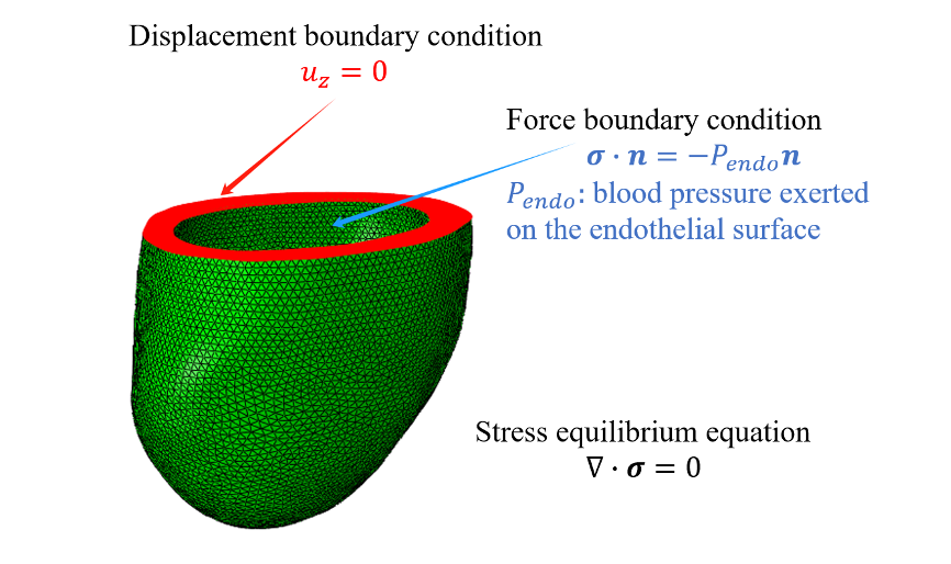
在该案例中，认为舒张期左心室被动力学是准静态的，因此认为该案例具有如下边界条件：

在整个几何计算域上需要满足 \(\nabla t=0\)，即：

\[ \begin{pmatrix} \frac{\partial t_{xx}}{\partial x}+\frac{\partial t_{xy}}{\partial y}+\frac{\partial t_{xz}}{\partial z}=0 \\ \frac{\partial t_{xy}}{\partial x}+\frac{\partial t_{yy}}{\partial y}+\frac{\partial t_{yz}}{\partial z}=0 \\ \frac{\partial t_{xz}}{\partial x}+\frac{\partial t_{yz}}{\partial y}+\frac{\partial t_{zz}}{\partial z}=0 \\ \end{pmatrix} \]

在心内膜表面需满足 \(tn=-P_{endo}n\)，这里 \(n\) 是心内膜表面的单位法线方向，\(P_{endo}=1.064kpa(8mmHg)\) 代表左心室空腔压力;
在心脏外膜上需满足 \(P_{epi}=0\);
在基面上需满足 \(u_{x,y,z}=0\)，即 \(u,v,w=0\)

3. 问题求解¶

接下来开始讲解如何将问题一步一步地转化为 PaddleScience 代码，用深度学习的方法求解该问题。为了快速理解 PaddleScience，接下来仅对模型构建、方程构建、计算域构建等关键步骤进行阐述，而其余细节请参考 API文档。

3.1 受力分析求解¶

3.1.1 模型构建¶

如上所述，每一个已知的坐标点 \((x, y, z)\) 都有对应的待求解的应变 \((u, v, w)\)，使用一个模型来预测：

\(u, v, w = f(x,y,z)\)

用 PaddleScience 代码表示如下：

# set model
model = ppsci.arch.MLP(**cfg.MODEL)

3.1.2 优化器构建¶

训练过程会调用优化器来更新模型参数，此处选择较为常用的 Adam 优化器，并配合使用机器学习中常用的 ExponentialDecay 学习率调整策略。

# set optimizer
lr_scheduler = ppsci.optimizer.lr_scheduler.ExponentialDecay(
    **cfg.TRAIN.lr_scheduler
)()
optimizer = ppsci.optimizer.Adam(lr_scheduler)(model)

3.1.3 方程构建¶

在 equation.py 文件中构建方程，对应的方程实例化代码如下：

# set equation
equation = {"Hooke": eq_func.Hooke(E=cfg.E, nu=cfg.nu, P=cfg.P, dim=3)}

3.1.4 计算域构建¶

本问题的几何区域由 stl 文件指定，按照本文档起始处"模型训练命令"下载并解压到 ./stl/ 文件夹下。

注意

使用 Mesh 类之前，必须先按照1.4.2 安装Mesh几何[可选]文档，安装好 open3d、pysdf、PyMesh 3 个几何依赖包。

然后通过 PaddleScience 内置的 STL 几何类 ppsci.geometry.Mesh 即可读取、解析几何文件，得到计算域，并获取几何结构边界：

# set geometry
heart = ppsci.geometry.Mesh(cfg.GEOM_PATH)
base = ppsci.geometry.Mesh(cfg.BASE_PATH)
endo = ppsci.geometry.Mesh(cfg.ENDO_PATH)
epi = ppsci.geometry.Mesh(cfg.EPI_PATH)
geom = {"geo": heart, "base": base, "endo": endo, "epi": epi}
# set bounds
BOUNDS_X, BOUNDS_Y, BOUNDS_Z = heart.bounds

3.1.5 超参数设定¶

接下来需要在配置文件中指定训练轮数，此处按实验经验，使用 200 轮训练轮数，每轮进行 1000 步优化。

  by_epoch: false
batch_size:

3.1.6 约束构建¶

本问题共涉及到2. 问题定义中的 4 个约束，在具体约束构建之前，可以先构建数据读取配置，以便后续构建多个约束时复用该配置。

# set dataloader config
train_dataloader_cfg = {
    "dataset": "NamedArrayDataset",
    "iters_per_epoch": cfg.TRAIN.iters_per_epoch,
    "sampler": {
        "name": "BatchSampler",
        "drop_last": True,
        "shuffle": True,
    },
    "num_workers": 1,
}

3.1.6.1 内部点约束¶

以作用在结构内部点的 InteriorConstraint 为例，代码如下：

interior = ppsci.constraint.InteriorConstraint(
    equation["Hooke"].equations,
    {"hooke_x": 0, "hooke_y": 0, "hooke_z": 0},
    geom["geo"],
    {**train_dataloader_cfg, "batch_size": cfg.TRAIN.batch_size.interior},
    ppsci.loss.MSELoss("mean"),
    criteria=lambda x, y, z: (
        (BOUNDS_X[0] < x)
        & (x < BOUNDS_X[1])
        & (BOUNDS_Y[0] < y)
        & (y < BOUNDS_Y[1])
        & (BOUNDS_Z[0] < z)
        & (z < BOUNDS_Z[1])
    ),
    weight_dict=cfg.TRAIN.weight.interior,
    name="INTERIOR",
)
data = ppsci.constraint.SupervisedConstraint(

InteriorConstraint 的第一个参数是方程（组）表达式，用于描述如何计算约束目标，此处填入在 3.1.3 方程构建章节中实例化好的 equation["Hooke"].equations；

第二个参数是约束变量的目标值，在本问题为 hooke_x, hooke_y, hooke_z 被优化至 0；

第三个参数是约束方程作用的计算域，此处填入在 3.1.4 计算域构建章节实例化好的 geom["geo"] 即可；

第四个参数是在计算域上的采样配置，此处设置 batch_size 为：

  bc_epi: { "traction": 0.2 }
  interior: { "hooke_x": 0.2, "hooke_y": 0.2, "hooke_z": 0.2 }
save_freq: 20
eval_freq: 20
eval_during_train: true

第五个参数是损失函数，此处选用常用的 MSE 函数，且 reduction 设置为 "mean"，即会将参与计算的所有数据点产生的损失项求均值；

第六个参数是几何点筛选，需要对 geo 上采样出的点进行筛选，此处传入一个 lambda 筛选函数即可，其接受点集构成的张量 x, y, z，返回布尔值张量，表示每个点是否符合筛选条件，不符合为 False，符合为 True，因为本案例结构来源于网络，参数不完全精确，因此增加 1e-1 作为可容忍的采样误差；

第七个参数是每个点参与损失计算时的权重；

第八个参数是约束条件的名字，需要给每一个约束条件命名，方便后续对其索引。此处命名为 "INTERIOR" 即可。

3.1.6.2 边界约束¶

参照 2. 问题定义分别为心内膜、心外膜和基面上的约束：

# set constraint
bc_base = ppsci.constraint.BoundaryConstraint(
    {"u": lambda d: d["u"], "v": lambda d: d["v"], "w": lambda d: d["w"]},
    {"u": 0, "v": 0, "w": 0},
    geom["base"],
    {**train_dataloader_cfg, "batch_size": cfg.TRAIN.batch_size.bc_base},
    ppsci.loss.MSELoss("mean"),
    weight_dict=cfg.TRAIN.weight.bc_base,
    name="BC_BASE",
)
bc_endo = ppsci.constraint.BoundaryConstraint(
    equation["Hooke"].equations,
    {"traction": -cfg.P},
    geom["endo"],
    {**train_dataloader_cfg, "batch_size": cfg.TRAIN.batch_size.bc_endo},
    ppsci.loss.MSELoss("mean"),
    weight_dict=cfg.TRAIN.weight.bc_endo,
    name="BC_ENDO",
)
bc_epi = ppsci.constraint.BoundaryConstraint(
    equation["Hooke"].equations,
    {"traction": 0},
    geom["epi"],
    {**train_dataloader_cfg, "batch_size": cfg.TRAIN.batch_size.bc_epi},
    ppsci.loss.MSELoss("mean"),
    weight_dict=cfg.TRAIN.weight.bc_epi,
    name="BC_EPI",
)

3.1.7 评估器构建¶

在训练过程中通常会按一定轮数间隔，用验证集（测试集）评估当前模型的训练情况，而验证集的数据来自外部 csv 文件，因此首先使用 ppsci.utils.reader 模块从 csv 文件中读取验证点集：

eval_data_dict = reader.load_csv_file(
    cfg.EVAL_CSV_PATH,
    ("x", "y", "z", "u", "v", "w"),
    {
        "x": "x",
        "y": "y",
        "z": "z",
        "u": "u",
        "v": "v",
        "w": "w",
    },
)

然后将其转换为字典并进行无量纲化和归一化，再将其包装成字典和 eval_dataloader_cfg（验证集dataloader配置，构造方式与 train_dataloader_cfg 类似）一起传递给 ppsci.validate.SupervisedValidator 构造评估器。

input_dict = {
    "x": eval_data_dict["x"],
    "y": eval_data_dict["y"],
    "z": eval_data_dict["z"],
}

label_dict = {
    "u": eval_data_dict["u"],
    "v": eval_data_dict["v"],
    "w": eval_data_dict["w"],
}
eval_dataloader_cfg = {
    "dataset": {
        "name": "NamedArrayDataset",
        "input": input_dict,
        "label": label_dict,
    },
    "num_workers": 1,
}
sup_validator = ppsci.validate.SupervisedValidator(
    {**eval_dataloader_cfg, "batch_size": cfg.EVAL.batch_size},
    ppsci.loss.MSELoss("mean"),
    {
        "u": lambda out: out["u"],
        "v": lambda out: out["v"],
        "w": lambda out: out["w"],
    },
    metric={"L2Rel": ppsci.metric.L2Rel()},
    name="ref_u_v_w",
)
validator = {sup_validator.name: sup_validator}

3.1.8 可视化器构建¶

在模型评估时，如果评估结果是可以可视化的数据，可以选择合适的可视化器来对输出结果进行可视化。

本文中的输入数据是评估器构建中准备好的输入字典 input_dict，输出数据是对应的 3 个预测的物理量，因此只需要将评估的输出数据保存成 vtu格式 文件，最后用可视化软件打开查看即可。代码如下：

# set visualizer(optional)
visualizer = {
    "visualize_u_v_w": ppsci.visualize.VisualizerVtu(
        input_dict,
        {
            "u": lambda out: out["u"],
            "v": lambda out: out["v"],
            "w": lambda out: out["w"],
        },
        batch_size=cfg.EVAL.batch_size,
        prefix="result_u_v_w",
    ),
}

3.1.8 模型训练¶

完成上述设置之后，只需要将上述实例化的对象按顺序传递给 ppsci.solver.Solver，然后启动训练：

# initialize solver
solver = ppsci.solver.Solver(
    model,
    constraint,
    optimizer=optimizer,
    equation=equation,
    validator=validator,
    visualizer=visualizer,
    cfg=cfg,
)

# train
solver.train()
# eval
solver.eval()
# visualize prediction after finished training
solver.visualize()

训练后调用 ppsci.solver.Solver.plot_loss_history 可以将训练中的 loss 画出：

# plot loss
solver.plot_loss_history(by_epoch=True)

3.1.9 模型评估与可视化¶

训练完成或下载预训练模型后，通过本文档起始处“模型评估命令”进行模型评估和可视化。

评估和可视化过程不需要进行优化器等构建，仅需构建模型、计算域、评估器（本案例不包括）、可视化器，然后按顺序传递给 ppsci.solver.Solver 启动评估和可视化：

# initialize solver
solver = ppsci.solver.Solver(
    model=model,
    validator=validator,
    visualizer=visualizer,
    cfg=cfg,
)

3.2 参数逆推求解¶

3.2.1 方程构建¶

本案例尝试在 PINN 框架下对心脏软组织复杂的超弹性本构关系进行建模和实现，在预设方程参数 \(E\) 未知的情况下，尝试通过部分数据，同时训练得到该未知参数的值。案例中依然使用 equation.py 文件中构建的方程，但需要将未知参数设为可学习变量，并传入方程：

# set equation
E = paddle.create_parameter(
    shape=[],
    dtype=paddle.get_default_dtype(),
    default_initializer=initializer.Constant(0.0),
)
equation = {"Hooke": eq_func.Hooke(E=E, nu=cfg.nu, P=cfg.P, dim=3)}

3.2.2 模型构建¶

模型设置与正问题相同：

# set models
model = ppsci.arch.MLP(**cfg.MODEL)

3.2.3 优化器构建¶

训练过程会调用优化器来更新模型参数，此处选择较为常用的 Adam 优化器，并配合使用机器学习中常用的 ExponentialDecay 学习率调整策略。在设置优化器时需要将方程中的可学习参数传递给优化器，来使该参数参与优化：

# set optimizer
lr_scheduler = ppsci.optimizer.lr_scheduler.ExponentialDecay(
    **cfg.TRAIN.lr_scheduler
)()
optimizer = ppsci.optimizer.Adam(lr_scheduler)((model,) + tuple(equation.values()))

3.2.4 其它设置¶

本问题的其它设置与正问题相似，在此不再赘述。

4. 完整代码¶

forward.py
# Copyright (c) 2024 PaddlePaddle Authors. All Rights Reserved.
#
# Licensed under the Apache License, Version 2.0 (the "License");
# you may not use this file except in compliance with the License.
# You may obtain a copy of the License at
#
#     http://www.apache.org/licenses/LICENSE-2.0
#
# Unless required by applicable law or agreed to in writing, software
# distributed under the License is distributed on an "AS IS" BASIS,
# WITHOUT WARRANTIES OR CONDITIONS OF ANY KIND, either express or implied.
# See the License for the specific language governing permissions and
# limitations under the License.

import equation as eq_func
import hydra
from omegaconf import DictConfig

import ppsci
from ppsci.utils import reader


def train(cfg: DictConfig):
    # set model
    model = ppsci.arch.MLP(**cfg.MODEL)

    # set optimizer
    lr_scheduler = ppsci.optimizer.lr_scheduler.ExponentialDecay(
        **cfg.TRAIN.lr_scheduler
    )()
    optimizer = ppsci.optimizer.Adam(lr_scheduler)(model)

    # set equation
    equation = {"Hooke": eq_func.Hooke(E=cfg.E, nu=cfg.nu, P=cfg.P, dim=3)}

    # set geometry
    heart = ppsci.geometry.Mesh(cfg.GEOM_PATH)
    base = ppsci.geometry.Mesh(cfg.BASE_PATH)
    endo = ppsci.geometry.Mesh(cfg.ENDO_PATH)
    epi = ppsci.geometry.Mesh(cfg.EPI_PATH)
    geom = {"geo": heart, "base": base, "endo": endo, "epi": epi}
    # set bounds
    BOUNDS_X, BOUNDS_Y, BOUNDS_Z = heart.bounds

    # set dataloader config
    train_dataloader_cfg = {
        "dataset": "NamedArrayDataset",
        "iters_per_epoch": cfg.TRAIN.iters_per_epoch,
        "sampler": {
            "name": "BatchSampler",
            "drop_last": True,
            "shuffle": True,
        },
        "num_workers": 1,
    }

    # set constraint
    bc_base = ppsci.constraint.BoundaryConstraint(
        {"u": lambda d: d["u"], "v": lambda d: d["v"], "w": lambda d: d["w"]},
        {"u": 0, "v": 0, "w": 0},
        geom["base"],
        {**train_dataloader_cfg, "batch_size": cfg.TRAIN.batch_size.bc_base},
        ppsci.loss.MSELoss("mean"),
        weight_dict=cfg.TRAIN.weight.bc_base,
        name="BC_BASE",
    )
    bc_endo = ppsci.constraint.BoundaryConstraint(
        equation["Hooke"].equations,
        {"traction": -cfg.P},
        geom["endo"],
        {**train_dataloader_cfg, "batch_size": cfg.TRAIN.batch_size.bc_endo},
        ppsci.loss.MSELoss("mean"),
        weight_dict=cfg.TRAIN.weight.bc_endo,
        name="BC_ENDO",
    )
    bc_epi = ppsci.constraint.BoundaryConstraint(
        equation["Hooke"].equations,
        {"traction": 0},
        geom["epi"],
        {**train_dataloader_cfg, "batch_size": cfg.TRAIN.batch_size.bc_epi},
        ppsci.loss.MSELoss("mean"),
        weight_dict=cfg.TRAIN.weight.bc_epi,
        name="BC_EPI",
    )
    interior = ppsci.constraint.InteriorConstraint(
        equation["Hooke"].equations,
        {"hooke_x": 0, "hooke_y": 0, "hooke_z": 0},
        geom["geo"],
        {**train_dataloader_cfg, "batch_size": cfg.TRAIN.batch_size.interior},
        ppsci.loss.MSELoss("mean"),
        criteria=lambda x, y, z: (
            (BOUNDS_X[0] < x)
            & (x < BOUNDS_X[1])
            & (BOUNDS_Y[0] < y)
            & (y < BOUNDS_Y[1])
            & (BOUNDS_Z[0] < z)
            & (z < BOUNDS_Z[1])
        ),
        weight_dict=cfg.TRAIN.weight.interior,
        name="INTERIOR",
    )
    data = ppsci.constraint.SupervisedConstraint(
        {
            "dataset": {
                "name": "IterableCSVDataset",
                "file_path": cfg.DATA_CSV_PATH,
                "input_keys": ("x", "y", "z"),
                "label_keys": ("u", "v", "w"),
            },
        },
        ppsci.loss.MSELoss("sum"),
        name="DATA",
    )

    # wrap constraints together
    constraint = {
        bc_base.name: bc_base,
        bc_endo.name: bc_endo,
        bc_epi.name: bc_epi,
        interior.name: interior,
        data.name: data,
    }

    # set validator
    eval_data_dict = reader.load_csv_file(
        cfg.EVAL_CSV_PATH,
        ("x", "y", "z", "u", "v", "w"),
        {
            "x": "x",
            "y": "y",
            "z": "z",
            "u": "u",
            "v": "v",
            "w": "w",
        },
    )

    input_dict = {
        "x": eval_data_dict["x"],
        "y": eval_data_dict["y"],
        "z": eval_data_dict["z"],
    }

    label_dict = {
        "u": eval_data_dict["u"],
        "v": eval_data_dict["v"],
        "w": eval_data_dict["w"],
    }
    eval_dataloader_cfg = {
        "dataset": {
            "name": "NamedArrayDataset",
            "input": input_dict,
            "label": label_dict,
        },
        "num_workers": 1,
    }
    sup_validator = ppsci.validate.SupervisedValidator(
        {**eval_dataloader_cfg, "batch_size": cfg.EVAL.batch_size},
        ppsci.loss.MSELoss("mean"),
        {
            "u": lambda out: out["u"],
            "v": lambda out: out["v"],
            "w": lambda out: out["w"],
        },
        metric={"L2Rel": ppsci.metric.L2Rel()},
        name="ref_u_v_w",
    )
    validator = {sup_validator.name: sup_validator}

    # set visualizer(optional)
    visualizer = {
        "visualize_u_v_w": ppsci.visualize.VisualizerVtu(
            input_dict,
            {
                "u": lambda out: out["u"],
                "v": lambda out: out["v"],
                "w": lambda out: out["w"],
            },
            batch_size=cfg.EVAL.batch_size,
            prefix="result_u_v_w",
        ),
    }

    # initialize solver
    solver = ppsci.solver.Solver(
        model,
        constraint,
        optimizer=optimizer,
        equation=equation,
        validator=validator,
        visualizer=visualizer,
        cfg=cfg,
    )

    # train
    solver.train()
    # eval
    solver.eval()
    # visualize prediction after finished training
    solver.visualize()
    # plot loss
    solver.plot_loss_history(by_epoch=True)


def evaluate(cfg: DictConfig):
    # set models
    model = ppsci.arch.MLP(**cfg.MODEL)

    # set validator
    eval_data_dict = reader.load_csv_file(
        cfg.EVAL_CSV_PATH,
        ("x", "y", "z", "u", "v", "w"),
        {
            "x": "x",
            "y": "y",
            "z": "z",
            "u": "u",
            "v": "v",
            "w": "w",
        },
    )

    input_dict = {
        "x": eval_data_dict["x"],
        "y": eval_data_dict["y"],
        "z": eval_data_dict["z"],
    }

    label_dict = {
        "u": eval_data_dict["u"],
        "v": eval_data_dict["v"],
        "w": eval_data_dict["w"],
    }
    eval_dataloader_cfg = {
        "dataset": {
            "name": "NamedArrayDataset",
            "input": input_dict,
            "label": label_dict,
        },
        "num_workers": 1,
    }
    sup_validator = ppsci.validate.SupervisedValidator(
        {**eval_dataloader_cfg, "batch_size": cfg.EVAL.batch_size},
        ppsci.loss.MSELoss("mean"),
        {
            "u": lambda out: out["u"],
            "v": lambda out: out["v"],
            "w": lambda out: out["w"],
        },
        metric={"L2Rel": ppsci.metric.L2Rel()},
        name="ref_u_v_w",
    )
    validator = {sup_validator.name: sup_validator}

    # set visualizer
    visualizer = {
        "visualize_u_v_w": ppsci.visualize.VisualizerVtu(
            input_dict,
            {
                "u": lambda out: out["u"],
                "v": lambda out: out["v"],
                "w": lambda out: out["w"],
            },
            batch_size=cfg.EVAL.batch_size,
            prefix="result_u_v_w",
        ),
    }

    # initialize solver
    solver = ppsci.solver.Solver(
        model=model,
        validator=validator,
        visualizer=visualizer,
        cfg=cfg,
    )

    # evaluate
    solver.eval()
    # visualize prediction
    solver.visualize()


@hydra.main(version_base=None, config_path="./conf", config_name="forward.yaml")
def main(cfg: DictConfig):
    if cfg.mode == "train":
        train(cfg)
    elif cfg.mode == "eval":
        evaluate(cfg)
    else:
        raise ValueError(f"cfg.mode should in ['train', 'eval'], but got '{cfg.mode}'")


if __name__ == "__main__":
    main()

inverse.py
# Copyright (c) 2024 PaddlePaddle Authors. All Rights Reserved.
#
# Licensed under the Apache License, Version 2.0 (the "License");
# you may not use this file except in compliance with the License.
# You may obtain a copy of the License at
#
#     http://www.apache.org/licenses/LICENSE-2.0
#
# Unless required by applicable law or agreed to in writing, software
# distributed under the License is distributed on an "AS IS" BASIS,
# WITHOUT WARRANTIES OR CONDITIONS OF ANY KIND, either express or implied.
# See the License for the specific language governing permissions and
# limitations under the License.

from os import path as osp

import equation as eq_func
import hydra
import numpy as np
import paddle
from omegaconf import DictConfig
from paddle.nn import initializer

import ppsci
from ppsci.metric import L2Rel
from ppsci.utils import logger
from ppsci.utils import reader


def train(cfg: DictConfig):
    # set equation
    E = paddle.create_parameter(
        shape=[],
        dtype=paddle.get_default_dtype(),
        default_initializer=initializer.Constant(0.0),
    )
    equation = {"Hooke": eq_func.Hooke(E=E, nu=cfg.nu, P=cfg.P, dim=3)}

    # set models
    model = ppsci.arch.MLP(**cfg.MODEL)

    # set optimizer
    lr_scheduler = ppsci.optimizer.lr_scheduler.ExponentialDecay(
        **cfg.TRAIN.lr_scheduler
    )()
    optimizer = ppsci.optimizer.Adam(lr_scheduler)((model,) + tuple(equation.values()))

    # set geometry
    heart = ppsci.geometry.Mesh(cfg.GEOM_PATH)
    base = ppsci.geometry.Mesh(cfg.BASE_PATH)
    endo = ppsci.geometry.Mesh(cfg.ENDO_PATH)
    epi = ppsci.geometry.Mesh(cfg.EPI_PATH)
    geom = {"geo": heart, "base": base, "endo": endo, "epi": epi}
    # set bounds
    BOUNDS_X, BOUNDS_Y, BOUNDS_Z = heart.bounds

    # set dataloader config
    train_dataloader_cfg = {
        "dataset": "NamedArrayDataset",
        "iters_per_epoch": cfg.TRAIN.iters_per_epoch,
        "sampler": {
            "name": "BatchSampler",
            "drop_last": True,
            "shuffle": True,
        },
        "num_workers": 1,
    }

    # set constraint
    bc_base = ppsci.constraint.BoundaryConstraint(
        {"u": lambda d: d["u"], "v": lambda d: d["v"], "w": lambda d: d["w"]},
        {"u": 0, "v": 0, "w": 0},
        geom["base"],
        {**train_dataloader_cfg, "batch_size": cfg.TRAIN.batch_size.bc_base},
        ppsci.loss.MSELoss("sum"),
        weight_dict=cfg.TRAIN.weight.bc_base,
        name="BC_BASE",
    )
    bc_endo = ppsci.constraint.BoundaryConstraint(
        equation["Hooke"].equations,
        {"traction_x": -cfg.P, "traction_y": -cfg.P, "traction_z": -cfg.P},
        geom["endo"],
        {**train_dataloader_cfg, "batch_size": cfg.TRAIN.batch_size.bc_endo},
        ppsci.loss.MSELoss("sum"),
        weight_dict=cfg.TRAIN.weight.bc_endo,
        name="BC_ENDO",
    )
    bc_epi = ppsci.constraint.BoundaryConstraint(
        equation["Hooke"].equations,
        {"traction_x": 0, "traction_y": 0, "traction_z": 0},
        geom["epi"],
        {**train_dataloader_cfg, "batch_size": cfg.TRAIN.batch_size.bc_epi},
        ppsci.loss.MSELoss("sum"),
        weight_dict=cfg.TRAIN.weight.bc_endo,
        name="BC_EPI",
    )
    interior = ppsci.constraint.InteriorConstraint(
        equation["Hooke"].equations,
        {"hooke_x": 0, "hooke_y": 0, "hooke_z": 0},
        geom["geo"],
        {**train_dataloader_cfg, "batch_size": cfg.TRAIN.batch_size.interior},
        ppsci.loss.MSELoss("sum"),
        criteria=lambda x, y, z: (
            (BOUNDS_X[0] < x)
            & (x < BOUNDS_X[1])
            & (BOUNDS_Y[0] < y)
            & (y < BOUNDS_Y[1])
            & (BOUNDS_Z[0] < z)
            & (z < BOUNDS_Z[1])
        ),
        weight_dict=cfg.TRAIN.weight.interior,
        name="INTERIOR",
    )
    data = ppsci.constraint.SupervisedConstraint(
        {
            "dataset": {
                "name": "IterableCSVDataset",
                "file_path": cfg.DATA_PATH,
                "input_keys": ("x", "y", "z"),
                "label_keys": ("u", "v", "w"),
            },
        },
        ppsci.loss.MSELoss("sum"),
        name="DATA",
    )

    # wrap constraints together
    constraint = {
        bc_base.name: bc_base,
        bc_endo.name: bc_endo,
        bc_epi.name: bc_epi,
        interior.name: interior,
        data.name: data,
    }

    # set validator
    eval_data_dict = reader.load_csv_file(
        cfg.DATA_PATH,
        ("x", "y", "z", "u", "v", "w"),
        {
            "x": "x",
            "y": "y",
            "z": "z",
            "u": "u",
            "v": "v",
            "w": "w",
        },
    )
    input_dict = {
        "x": eval_data_dict["x"],
        "y": eval_data_dict["y"],
        "z": eval_data_dict["z"],
    }
    label_dict = {
        "u": eval_data_dict["u"],
        "v": eval_data_dict["v"],
        "w": eval_data_dict["w"],
    }
    eval_dataloader_cfg = {
        "dataset": {
            "name": "NamedArrayDataset",
            "input": input_dict,
            "label": label_dict,
        },
        "num_workers": 1,
    }
    sup_validator = ppsci.validate.SupervisedValidator(
        {**eval_dataloader_cfg, "batch_size": cfg.EVAL.batch_size},
        ppsci.loss.MSELoss("mean"),
        {
            "u": lambda out: out["u"],
            "v": lambda out: out["v"],
            "w": lambda out: out["w"],
        },
        metric={"L2Rel": ppsci.metric.L2Rel()},
        name="ref_u_v_w",
    )

    fake_input = np.full((1, 1), 1, dtype=np.float32)
    E_label = np.full((1, 1), cfg.E, dtype=np.float32)
    param_validator = ppsci.validate.SupervisedValidator(
        {
            "dataset": {
                "name": "NamedArrayDataset",
                "input": {
                    "x": fake_input,
                    "y": fake_input,
                    "z": fake_input,
                },
                "label": {"E": E_label},
            },
            "batch_size": 1,
            "num_workers": 1,
        },
        ppsci.loss.MSELoss("mean"),
        {
            "E": lambda out: E.reshape([1, 1]),
        },
        metric={"L2Rel": ppsci.metric.L2Rel()},
        name="param_E",
    )

    validator = {
        sup_validator.name: sup_validator,
        param_validator.name: param_validator,
    }

    # set visualizer(optional)
    visualizer = {
        "visualize_u_v_w": ppsci.visualize.VisualizerVtu(
            input_dict,
            {
                "u": lambda out: out["u"],
                "v": lambda out: out["v"],
                "w": lambda out: out["w"],
            },
            batch_size=cfg.EVAL.batch_size,
            prefix="result_u_v_w",
        ),
    }

    # initialize solver
    solver = ppsci.solver.Solver(
        model,
        constraint,
        optimizer=optimizer,
        equation=equation,
        validator=validator,
        visualizer=visualizer,
        cfg=cfg,
    )

    # train
    solver.train()
    # eval
    solver.eval()
    # visualize prediction after finished training
    solver.visualize()
    # plot loss
    solver.plot_loss_history(by_epoch=True)

    # save parameter E separately
    paddle.save({"E": E}, osp.join(cfg.output_dir, "param_E.pdparams"))


def evaluate(cfg: DictConfig):
    # set models
    model = ppsci.arch.MLP(**cfg.MODEL)

    # set geometry
    heart = ppsci.geometry.Mesh(cfg.GEOM_PATH)
    base = ppsci.geometry.Mesh(cfg.BASE_PATH)
    endo = ppsci.geometry.Mesh(cfg.ENDO_PATH)
    epi = ppsci.geometry.Mesh(cfg.EPI_PATH)
    # test = ppsci.geometry.Cuboid((0, 0, 0), (1, 1, 1))
    geom = {"geo": heart, "base": base, "endo": endo, "epi": epi}
    # set bounds
    BOUNDS_X, BOUNDS_Y, BOUNDS_Z = heart.bounds

    # set validator
    eval_data_dict = reader.load_csv_file(
        cfg.DATA_PATH,
        ("x", "y", "z", "u", "v", "w"),
        {
            "x": "x",
            "y": "y",
            "z": "z",
            "u": "u",
            "v": "v",
            "w": "w",
        },
    )
    input_dict = {
        "x": eval_data_dict["x"],
        "y": eval_data_dict["y"],
        "z": eval_data_dict["z"],
    }
    label_dict = {
        "u": eval_data_dict["u"],
        "v": eval_data_dict["v"],
        "w": eval_data_dict["w"],
    }
    eval_dataloader_cfg = {
        "dataset": {
            "name": "NamedArrayDataset",
            "input": input_dict,
            "label": label_dict,
        },
        "num_workers": 1,
    }
    sup_validator = ppsci.validate.SupervisedValidator(
        {**eval_dataloader_cfg, "batch_size": cfg.EVAL.batch_size},
        ppsci.loss.MSELoss("mean"),
        {
            "u": lambda out: out["u"],
            "v": lambda out: out["v"],
            "w": lambda out: out["w"],
        },
        metric={"L2Rel": ppsci.metric.L2Rel()},
        name="ref_u_v_w",
    )
    validator = {sup_validator.name: sup_validator}

    # set visualizer(optional)
    # add inferencer data endo
    samples_endo = geom["endo"].sample_boundary(
        cfg.EVAL.num_vis,
        criteria=lambda x, y, z: (
            (BOUNDS_X[0] < x)
            & (x < BOUNDS_X[1])
            & (BOUNDS_Y[0] < y)
            & (y < BOUNDS_Y[1])
            & (BOUNDS_Z[0] < z)
            & (z < BOUNDS_Z[1])
        ),
    )
    pred_input_dict_endo = {
        "x": samples_endo["x"],
        "y": samples_endo["y"],
        "z": samples_endo["z"],
    }
    visualizer_endo = ppsci.visualize.VisualizerVtu(
        pred_input_dict_endo,
        {
            "u": lambda out: out["u"],
            "v": lambda out: out["v"],
            "w": lambda out: out["w"],
        },
        prefix="vtu_u_v_w_endo",
    )
    # add inferencer data epi
    samples_epi = geom["epi"].sample_boundary(
        cfg.EVAL.num_vis,
        criteria=lambda x, y, z: (
            (BOUNDS_X[0] < x)
            & (x < BOUNDS_X[1])
            & (BOUNDS_Y[0] < y)
            & (y < BOUNDS_Y[1])
            & (BOUNDS_Z[0] < z)
            & (z < BOUNDS_Z[1])
        ),
    )
    pred_input_dict_epi = {
        "x": samples_epi["x"],
        "y": samples_epi["y"],
        "z": samples_epi["z"],
    }
    visualizer_epi = ppsci.visualize.VisualizerVtu(
        pred_input_dict_epi,
        {
            "u": lambda out: out["u"],
            "v": lambda out: out["v"],
            "w": lambda out: out["w"],
        },
        prefix="vtu_u_v_w_epi",
    )
    # add inferencer data
    samples_geom = geom["geo"].sample_interior(
        cfg.EVAL.num_vis,
        criteria=lambda x, y, z: (
            (BOUNDS_X[0] < x)
            & (x < BOUNDS_X[1])
            & (BOUNDS_Y[0] < y)
            & (y < BOUNDS_Y[1])
            & (BOUNDS_Z[0] < z)
            & (z < BOUNDS_Z[1])
        ),
    )
    pred_input_dict_geom = {
        "x": samples_geom["x"],
        "y": samples_geom["y"],
        "z": samples_geom["z"],
    }
    visualizer_geom = ppsci.visualize.VisualizerVtu(
        pred_input_dict_geom,
        {
            "u": lambda out: out["u"],
            "v": lambda out: out["v"],
            "w": lambda out: out["w"],
        },
        prefix="vtu_u_v_w_geom",
    )

    # wrap visualizers together
    visualizer = {
        "vis_eval_endo": visualizer_endo,
        "visualizer_epi": visualizer_epi,
        "vis_eval_geom": visualizer_geom,
    }

    # initialize solver
    solver = ppsci.solver.Solver(
        model=model,
        validator=validator,
        visualizer=visualizer,
        cfg=cfg,
    )
    # evaluate
    solver.eval()
    # visualize prediction after finished training
    solver.visualize()

    # evaluate E
    E_truth = paddle.to_tensor(cfg.E, dtype=paddle.get_default_dtype()).reshape([1, 1])
    E_pred = paddle.load(cfg.EVAL.param_E_path)["E"].reshape([1, 1])
    l2_error = L2Rel()({"E": E_pred}, {"E": E_truth})["E"]
    logger.info(
        f"E_truth: {cfg.E}, E_pred: {float(E_pred)}, L2_Error: {float(l2_error)}"
    )


@hydra.main(version_base=None, config_path="./conf", config_name="inverse.yaml")
def main(cfg: DictConfig):
    if cfg.mode == "train":
        train(cfg)
    elif cfg.mode == "eval":
        evaluate(cfg)
    else:
        raise ValueError(f"cfg.mode should in ['train', 'eval'], but got '{cfg.mode}'")


if __name__ == "__main__":
    main()

equation.py
# Copyright (c) 2024 PaddlePaddle Authors. All Rights Reserved.

# Licensed under the Apache License, Version 2.0 (the "License");
# you may not use this file except in compliance with the License.
# You may obtain a copy of the License at

#     http://www.apache.org/licenses/LICENSE-2.0

# Unless required by applicable law or agreed to in writing, software
# distributed under the License is distributed on an "AS IS" BASIS,
# WITHOUT WARRANTIES OR CONDITIONS OF ANY KIND, either express or implied.
# See the License for the specific language governing permissions and
# limitations under the License.

from __future__ import annotations

from typing import Optional
from typing import Tuple
from typing import Union

import paddle
import sympy as sp

from ppsci.equation.pde import base


class Hooke(base.PDE):
    r"""equations for umbrella opening force.
    Use either (E, nu) or (lambda_, mu) to define the material properties.

    $$
    \begin{pmatrix}
        t_{xx} \\ t_{yy} \\ t_{zz} \\ t_{xy} \\ t_{xz} \\ t_{yz} \\
    \end{pmatrix}
    =
    \begin{bmatrix}
        \frac{1}{E} & -\frac{\nu}{E} & -\frac{\nu}{E} & 0 & 0 & 0 \\
        -\frac{\nu}{E} & \frac{1}{E} & -\frac{\nu}{E} & 0 & 0 & 0 \\
        -\frac{\nu}{E} & -\frac{\nu}{E} & \frac{1}{E} & 0 & 0 & 0 \\
        0 & 0 & 0 & \frac{1}{G} & 0 & 0 \\
        0 & 0 & 0 & 0 & \frac{1}{G} & 0 \\
        0 & 0 & 0 & 0 & 0 & \frac{1}{G}  \\
    \end{bmatrix}
    \begin{pmatrix}
        \varepsilon _{xx} \\ \varepsilon _{yy} \\ \varepsilon _{zz} \\ \varepsilon _{xy} \\ \varepsilon _{xz} \\ \varepsilon _{yz} \\
    \end{pmatrix}
    $$

    Args:
        E (paddle.base.framework.EagerParamBase): The Young's modulus. Learnable parameter.
        nu (Union[float, str]): The Poisson's ratio.
        P (Union[float, str]): Left ventricular cavity pressure.
        dim (int, optional): Dimension of the linear elasticity (2 or 3). Defaults to 3.
        time (bool, optional): Whether contains time data. Defaults to False.
        detach_keys (Optional[Tuple[str, ...]]): Keys used for detach during computing.
            Defaults to None.


    Examples:
        >>> import ppsci
        >>> E = paddle.create_parameter(
        ...     shape=[],
        ...     dtype=paddle.get_default_dtype(),
        ...     default_initializer=initializer.Constant(),
        ... )
        >>> pde = ppsci.equation.Hooke(
        ...     E=E, nu=cfg.nu, P=cfg.P, dim=3
        ... )
    """

    def __init__(
        self,
        E: Union[float, str, paddle.base.framework.EagerParamBase],
        nu: Union[float, str],
        P: Union[float, str],
        dim: int = 3,
        time: bool = False,
        detach_keys: Optional[Tuple[str, ...]] = None,
    ):
        super().__init__()
        self.detach_keys = detach_keys
        self.dim = dim
        self.time = time

        t, x, y, z = self.create_symbols("t x y z")
        normal_x, normal_y, normal_z = self.create_symbols("normal_x normal_y normal_z")
        invars = (x, y)
        if time:
            invars = (t,) + invars
        if self.dim == 3:
            invars += (z,)

        u = self.create_function("u", invars)
        v = self.create_function("v", invars)
        w = self.create_function("w", invars) if dim == 3 else sp.Number(0)

        if isinstance(nu, str):
            nu = self.create_function(nu, invars)
        if isinstance(P, str):
            P = self.create_function(P, invars)
        if isinstance(E, str):
            E = self.create_function(E, invars)
            self.E = E
        elif isinstance(E, paddle.base.framework.EagerParamBase):
            self.E = E
            self.learnable_parameters.append(self.E)
            E = self.create_symbols(self.E.name)

        self.nu = nu
        self.P = P

        # compute sigma
        sigma_xx = u.diff(x)
        sigma_yy = v.diff(y)
        sigma_zz = w.diff(z) if dim == 3 else sp.Number(0)
        sigma_xy = 0.5 * (u.diff(y) + v.diff(x))
        sigma_xz = 0.5 * (u.diff(z) + w.diff(x)) if dim == 3 else sp.Number(0)
        sigma_yz = 0.5 * (v.diff(z) + w.diff(y)) if dim == 3 else sp.Number(0)

        # compute stress tensor t
        G = E / (2 * (1 + nu))
        e = sigma_xx + sigma_yy + sigma_zz
        t_xx = 2 * G * (sigma_xx + nu / (1 - 2 * nu) * e)
        t_yy = 2 * G * (sigma_yy + nu / (1 - 2 * nu) * e)
        t_zz = 2 * G * (sigma_zz + nu / (1 - 2 * nu) * e)
        t_xy = 2 * sigma_xy * G
        t_xz = 2 * sigma_xz * G
        t_yz = 2 * sigma_yz * G

        # compute stress
        hooke_x = t_xx.diff(x) + t_xy.diff(y) + t_xz.diff(z)
        hooke_y = t_xy.diff(x) + t_yy.diff(y) + t_yz.diff(z)
        hooke_z = t_xz.diff(x) + t_yz.diff(y) + t_zz.diff(z)

        # compute traction splitly
        traction_x = t_xx * normal_x + t_xy * normal_y + t_xz * normal_z + P * normal_x
        traction_y = t_xy * normal_x + t_yy * normal_y + t_yz * normal_z + P * normal_y
        traction_z = t_xz * normal_x + t_yz * normal_y + t_zz * normal_z + P * normal_z

        # compute traction
        traction_x_ = t_xx * normal_x + t_xy * normal_y + t_xz * normal_z
        traction_y_ = t_xy * normal_x + t_yy * normal_y + t_yz * normal_z
        traction_z_ = t_xz * normal_x + t_yz * normal_y + t_zz * normal_z

        traction = (
            traction_x_ * normal_x + traction_y_ * normal_y + traction_z_ * normal_z
        )

        # add hooke equations
        self.add_equation("hooke_x", hooke_x)
        self.add_equation("hooke_y", hooke_y)
        if self.dim == 3:
            self.add_equation("hooke_z", hooke_z)

        # add traction equations
        self.add_equation("traction_x", traction_x)
        self.add_equation("traction_y", traction_y)
        if self.dim == 3:
            self.add_equation("traction_z", traction_z)

        # add combined traction equations
        self.add_equation("traction", traction)

        self._apply_detach()

5. 结果展示¶

5.1 受力分析求解¶

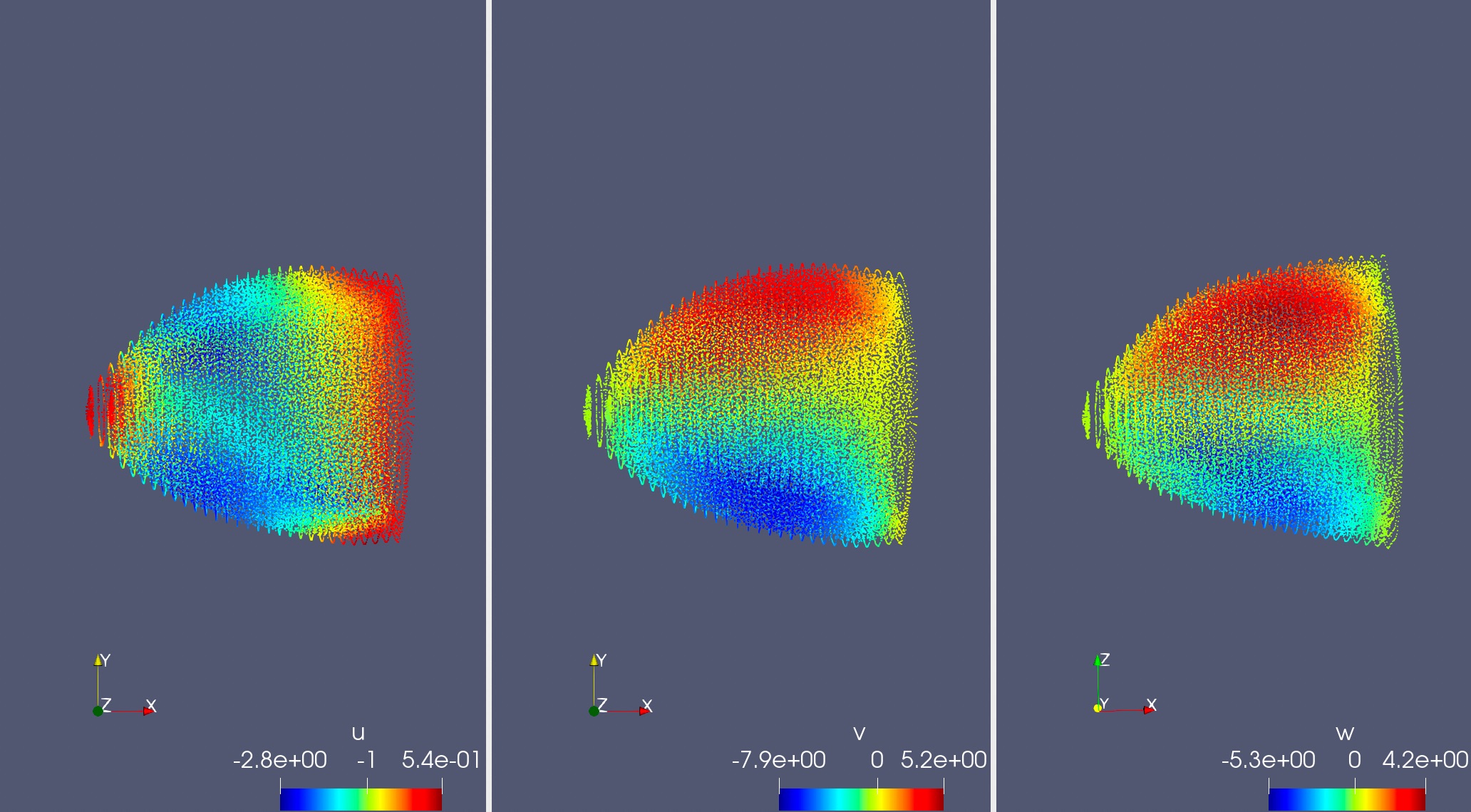
下面展示了当力的方向为 x 正方向时 3 个方向的应变 \(u, v, w\) 的模型预测结果，结果基本符合认知。

5.2 参数逆推求解¶

下面展示了可学习方程参数 \(E\) 的模型预测结果，误差在 5% 左右。

data	E
outs	9
label	9.44778