CVit(Advection)

AI Studio快速体验

Note

运行模型前请在 Zhengyu-Huang/Operator-Learning 中下载 adv_a0.npy 和 adv_aT.npy 两个文件，并将其放在 ./examples/adv/data/ 文件夹下。

模型训练命令模型评估命令模型导出命令模型推理命令

python adv_cvit.py

python adv_cvit.py mode=eval EVAL.pretrained_model_path=https://paddle-org.bj.bcebos.com/paddlescience/models/cvit/adv_cvit_pretrained.pdparams

python adv_cvit.py mode=export

python adv_cvit.py mode=infer

预训练模型	指标
adv_cvit_pretrained.pdparams	L2 error(mean): 0.028 L2 error(median): 0.022 L2 error(max): 0.166 L2 error(min): 0.0015

1. 背景简介

sciml 领域所使用的模型现阶段与CV、NLP领域的先进模型有较大差别，并没有很好地利用好这些先进模型所提供的优势。因此论文作者首先提出了一个算子学习的统一视角，按照 Global conditioning 和 Local Conditioning 分别对 DeepONet、FNO、GNO 等模型进行了归纳与总结，然后基于目前广泛应用于CV、NLP领域的 Transformer 结构设计了一种 Global conditioning 的模型 CVit。相比以往的算子学习模型，参数量更小，精度更高。

模型结构如下图所示：

2. 问题定义

CVit 作为一种算子学习模型，以输入函数 \(u\)、函数 \(s\) 的查询点 query coordinate \(y\) 为输入，输出经过算子映射后的函数，在查询点 \(y\) 处的函数值 \(s(y)\)。

本问题求解如下方程：

Formulation The 1D advection equation in \(\Omega=[0,1)\) is

\[ \begin{aligned} & \frac{\partial u}{\partial t}+c \frac{\partial u}{\partial x}=0 \quad x \in \Omega, \\ & u(0)=u_0 \end{aligned} \]

where \(c=1\) is the constant advection speed, and periodic boundary conditions are imposed. We are interested in the map from the initial \(u_0\) to solution \(u(\cdot, T)\) at \(T=0.5\). The initial condition \(u_0\) is assumed to be

\[ u_0=-1+2 \mathbb{1}\left\{\tilde{u_0} \geq 0\right\} \]

where \(\widetilde{u_0}\) a centered Gaussian

\[ \widetilde{u_0} \sim \mathbb{N}(0, \mathrm{C}) \quad \text { and } \quad \mathrm{C}=\left(-\Delta+\tau^2\right)^{-d} \text {; } \]

3. 问题求解

接下来开始讲解如何将问题一步一步地转化为 PaddleScience 代码，用深度学习的方法求解该问题。 为了快速理解 PaddleScience，接下来仅对模型构建、方程构建、计算域构建等关键步骤进行阐述，而其余细节请参考 API文档。

3.1 模型构建

在本问题中，对于每一个函数 \(u\)，其经过算子学习模型映射到 \(s\) 后，在 \(y\) 上都有对应的标签 \(s(y)\)，因此在这里使用 CVit 来表示 \((u, y)\) 到 \(s(y)\) 的映射关系：

\[ s(y) = G(u)(y) \]

上式中 \(G(u)\) 即为 CVit 模型本身，用 PaddleScience 代码表示如下

# set model
model = ppsci.arch.CVit1D(**cfg.MODEL)

为了在计算时，准确快速地访问具体变量的值，在这里指定网络模型的输入变量名是 ("u", "y")，输出变量名是 ("s")，这些命名与后续代码保持一致。

接着通过指定 CVit 的输入维度、坐标维度、输出维度、模型层数等超参数，就可实例化出了一个 model

# model settings
MODEL:
  input_keys: [u, y]
  output_keys: [s]
  in_dim: 1
  coords_dim: 1
  spatial_dims: 200
  patch_size: [4]
  grid_size: [200]
  latent_dim: 256
  emb_dim: 256
  depth: 6
  num_heads: 16
  dec_emb_dim: 256
  dec_num_heads: 16
  dec_depth: 1
  num_mlp_layers: 1
  mlp_ratio: 1
  out_dim: 1
  layer_norm_eps: 1.0e-5
  embedding_type: grid

3.2 数据准备

本问题中的数据储存在 adv_a0.py 和 adv_aT.py 文件中，将数据随机打乱后，取前 20000 个数据为训练数据，后 10000 个为测试数据。

        return tvd

    tvd = compute_tvd(np.squeeze(pred, axis=-1), label, 1 / 199)
    logger.message(
        f"mean: {np.mean(tvd)}, "
        f"median: {np.median(tvd)}, "
        f"max: {np.amax(tvd)}, "
        f"min: {np.amin(tvd)}"
    )

    best_idx = np.argmin(tvd)
    worst_idx = np.argmax(tvd)
    logger.message(f"best: {best_idx}, worst: {worst_idx}")

    idx = worst_idx
    x = np.linspace(0, 1, 200)
    plt.plot(x, pred[idx], "r--")
    plt.plot(x, label[idx], "b-")
    plt.title(f"CViT (TV: {tvd[idx]:.2f})")
    plt.xlabel("$y$")
    plt.ylim([-1.4, 1.4])

    plt.tight_layout()
    plt.savefig(osp.join(output_dir, "adv_cvit.png"))
    logger.message(f"Result saved to: {osp.join(output_dir, 'adv_cvit.png')}")


def train(cfg: DictConfig):
    # set model
    model = ppsci.arch.CVit1D(**cfg.MODEL)

    # prepare dataset
    inputs = np.load(osp.join(cfg.DATA_DIR, "adv_a0.npy")).astype(dtype)
    outputs = np.load(osp.join(cfg.DATA_DIR, "adv_aT.npy")).astype(dtype)
    grid = np.linspace(0, 1, inputs.shape[0], dtype=dtype)
    grid = einops.repeat(grid, "i -> i b", b=inputs.shape[1])

    ## swapping the first two axes:
    inputs = einops.rearrange(inputs, "i j -> j i 1")  # (40000, 200, 1)
    outputs = einops.rearrange(outputs, "i j -> j i")  # (40000, 200)
    grid = einops.rearrange(grid, "i j -> j i 1")  # (40000, 200, 1)

    idx = np.random.permutation(inputs.shape[0])
    n_train = 20000
    n_test = 10000
    inputs_train, outputs_train, grid_train = (
        inputs[idx[:n_train]],
        outputs[idx[:n_train]],
        grid[idx[:n_train]],
    )

3.3 约束构建

3.3.1 监督约束

在训练时，随机选取 batch_size 组来自 \(u\) 上的数据、并同时随机选取 query_point 个 \(y\) 坐标，如此构成了训练输入数据，标签数据则从 \(s\) 中随机选取同样的 batch_size x query_point 个标签点。

# set constraint
def gen_input_batch_train():
    batch_idx = np.random.randint(0, inputs_train.shape[0], [cfg.TRAIN.batch_size])
    grid_idx = np.sort(
        np.random.randint(0, inputs_train.shape[1], [cfg.TRAIN.grid_size])
    )
    return {
        "u": inputs_train[batch_idx],
        "y": grid_train[batch_idx][:, grid_idx],
        "batch_idx": batch_idx,
        "grid_idx": grid_idx,
    }

def gen_label_batch_train(input_batch):
    batch_idx, grid_idx = input_batch.pop("batch_idx"), input_batch.pop("grid_idx")
    return {
        "s": outputs_train[batch_idx][:, grid_idx, None],
    }

sup_constraint = ppsci.constraint.SupervisedConstraint(
    {
        "dataset": {
            "name": "ContinuousNamedArrayDataset",
            "input": gen_input_batch_train,
            "label": gen_label_batch_train,
        },
    },
    output_expr={"s": lambda out: out["s"]},
    loss=ppsci.loss.MSELoss("mean"),
    name="Sup",
)
# wrap constraints together
constraint = {sup_constraint.name: sup_constraint}

SupervisedConstraint 的第一个参数是用于训练的数据配置，我们使用 ContinuousNamedArrayDataset 作为数据集类型，并且传入自定义的gen_input_batch_train和gen_label_batch_train来完成上述的训练输入、标签样本的随机选取过程；

第二个参数是该约束的计算表达式，我们只需要计算 \(s\) 即可，因此填入一个不做任何处理，直接取出模型输出结果"s"的匿名表达式；

第三个参数是损失函数，此处选用 MSELoss 函数；

第四个参数是约束条件的名字，需要给每一个约束条件命名，方便后续对其索引。此处命名为 "Sup" 即可。

3.4 超参数设定

接下来需要指定训练轮数和学习率，此处按实验经验，使用 200000 轮训练轮数，所以总共为，初始学习率为 0.0001，全局梯度裁剪系数为 1.0，权重衰减为 1e-5，并且每 1 轮训练过程中都进行模型平均 EMA。

# training settings
TRAIN:
  epochs: 200000
  iters_per_epoch: 1
  save_freq: 10000
  eval_during_train: false
  eval_freq: 5
  lr_scheduler:
    epochs: ${TRAIN.epochs}
    iters_per_epoch: ${TRAIN.iters_per_epoch}
    learning_rate: 1.0e-4
    gamma: 0.95
    decay_steps: 1000
    by_epoch: false
  weight_decay: 1.0e-5
  grad_clip: 1.0
  batch_size: 256
  grid_size: 128
  pretrained_model_path: null
  checkpoint_path: null
  ema:
    use_ema: true
    decay: 0.999
    avg_freq: 1

3.5 优化器构建

训练过程会调用优化器来更新模型参数，此处选择较 AdamW 优化器，并配合使用机器学习中常用的 ExponentialDecay 学习率调整策略。

# set optimizer
lr_scheduler = ppsci.optimizer.lr_scheduler.ExponentialDecay(
    **cfg.TRAIN.lr_scheduler
)()
optimizer = ppsci.optimizer.AdamW(
    lr_scheduler,
    weight_decay=cfg.TRAIN.weight_decay,
    grad_clip=paddle.nn.ClipGradByGlobalNorm(cfg.TRAIN.grad_clip),
)(model)

3.6 模型训练、评估

完成上述设置之后，只需要将上述实例化的对象按顺序传递给 ppsci.solver.Solver，然后启动训练、评估。

# initialize solver
solver = ppsci.solver.Solver(
    model,
    constraint,
    optimizer=optimizer,
    cfg=cfg,
)
# train model
solver.train()
# visualzie result on ema model
solver.ema_model.apply_shadow()
pred_s = solver.predict(
    {"u": inputs_test, "y": grid_test},
    batch_size=cfg.EVAL.batch_size,
    return_numpy=True,
)["s"]

plot_result(pred_s, outputs_test, cfg.output_dir)
solver.ema_model.restore()

4. 完整代码

"""
Reference: https://github.com/PredictiveIntelligenceLab/cvit/tree/main/adv/
"""

from os import path as osp

import einops
import hydra
import matplotlib.pyplot as plt
import numpy as np
import paddle
from omegaconf import DictConfig

import ppsci
from ppsci.utils import logger

dtype = paddle.get_default_dtype()


def plot_result(pred: np.ndarray, label: np.ndarray, output_dir: str):
    def compute_tvd(f, g, dx):
        assert f.shape == g.shape
        df = np.abs(np.diff(f, axis=1))
        dg = np.abs(np.diff(g, axis=1))

        tvd = np.sum(np.abs(df - dg), axis=1) * dx
        return tvd

    tvd = compute_tvd(np.squeeze(pred, axis=-1), label, 1 / 199)
    logger.message(
        f"mean: {np.mean(tvd)}, "
        f"median: {np.median(tvd)}, "
        f"max: {np.amax(tvd)}, "
        f"min: {np.amin(tvd)}"
    )

    best_idx = np.argmin(tvd)
    worst_idx = np.argmax(tvd)
    logger.message(f"best: {best_idx}, worst: {worst_idx}")

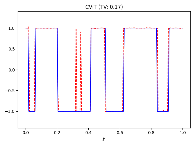
    idx = worst_idx
    x = np.linspace(0, 1, 200)
    plt.plot(x, pred[idx], "r--")
    plt.plot(x, label[idx], "b-")
    plt.title(f"CViT (TV: {tvd[idx]:.2f})")
    plt.xlabel("$y$")
    plt.ylim([-1.4, 1.4])

    plt.tight_layout()
    plt.savefig(osp.join(output_dir, "adv_cvit.png"))
    logger.message(f"Result saved to: {osp.join(output_dir, 'adv_cvit.png')}")


def train(cfg: DictConfig):
    # set model
    model = ppsci.arch.CVit1D(**cfg.MODEL)

    # prepare dataset
    inputs = np.load(osp.join(cfg.DATA_DIR, "adv_a0.npy")).astype(dtype)
    outputs = np.load(osp.join(cfg.DATA_DIR, "adv_aT.npy")).astype(dtype)
    grid = np.linspace(0, 1, inputs.shape[0], dtype=dtype)
    grid = einops.repeat(grid, "i -> i b", b=inputs.shape[1])

    ## swapping the first two axes:
    inputs = einops.rearrange(inputs, "i j -> j i 1")  # (40000, 200, 1)
    outputs = einops.rearrange(outputs, "i j -> j i")  # (40000, 200)
    grid = einops.rearrange(grid, "i j -> j i 1")  # (40000, 200, 1)

    idx = np.random.permutation(inputs.shape[0])
    n_train = 20000
    n_test = 10000
    inputs_train, outputs_train, grid_train = (
        inputs[idx[:n_train]],
        outputs[idx[:n_train]],
        grid[idx[:n_train]],
    )
    inputs_test, outputs_test, grid_test = (
        inputs[idx[-n_test:]],
        outputs[idx[-n_test:]],
        grid[idx[-n_test:]],
    )

    # set constraint
    def gen_input_batch_train():
        batch_idx = np.random.randint(0, inputs_train.shape[0], [cfg.TRAIN.batch_size])
        grid_idx = np.sort(
            np.random.randint(0, inputs_train.shape[1], [cfg.TRAIN.grid_size])
        )
        return {
            "u": inputs_train[batch_idx],
            "y": grid_train[batch_idx][:, grid_idx],
            "batch_idx": batch_idx,
            "grid_idx": grid_idx,
        }

    def gen_label_batch_train(input_batch):
        batch_idx, grid_idx = input_batch.pop("batch_idx"), input_batch.pop("grid_idx")
        return {
            "s": outputs_train[batch_idx][:, grid_idx, None],
        }

    sup_constraint = ppsci.constraint.SupervisedConstraint(
        {
            "dataset": {
                "name": "ContinuousNamedArrayDataset",
                "input": gen_input_batch_train,
                "label": gen_label_batch_train,
            },
        },
        output_expr={"s": lambda out: out["s"]},
        loss=ppsci.loss.MSELoss("mean"),
        name="Sup",
    )
    # wrap constraints together
    constraint = {sup_constraint.name: sup_constraint}

    # set optimizer
    lr_scheduler = ppsci.optimizer.lr_scheduler.ExponentialDecay(
        **cfg.TRAIN.lr_scheduler
    )()
    optimizer = ppsci.optimizer.AdamW(
        lr_scheduler,
        weight_decay=cfg.TRAIN.weight_decay,
        grad_clip=paddle.nn.ClipGradByGlobalNorm(cfg.TRAIN.grad_clip),
    )(model)

    # initialize solver
    solver = ppsci.solver.Solver(
        model,
        constraint,
        optimizer=optimizer,
        cfg=cfg,
    )
    # train model
    solver.train()
    # visualzie result on ema model
    solver.ema_model.apply_shadow()
    pred_s = solver.predict(
        {"u": inputs_test, "y": grid_test},
        batch_size=cfg.EVAL.batch_size,
        return_numpy=True,
    )["s"]

    plot_result(pred_s, outputs_test, cfg.output_dir)
    solver.ema_model.restore()


def evaluate(cfg: DictConfig):
    # set model
    model = ppsci.arch.CVit1D(**cfg.MODEL)

    # prepare dataset
    inputs = np.load(osp.join(cfg.DATA_DIR, "adv_a0.npy")).astype(dtype)
    outputs = np.load(osp.join(cfg.DATA_DIR, "adv_aT.npy")).astype(dtype)
    grid = np.linspace(0, 1, inputs.shape[0], dtype=dtype)
    grid = einops.repeat(grid, "i -> i b", b=inputs.shape[1])

    ## swapping the first two axes:
    inputs = einops.rearrange(inputs, "i j -> j i 1")  # (40000, 200, 1)
    outputs = einops.rearrange(outputs, "i j -> j i")  # (40000, 200)
    grid = einops.rearrange(grid, "i j -> j i 1")  # (40000, 200, 1)

    idx = np.random.permutation(inputs.shape[0])
    n_test = 10000
    inputs_test, outputs_test, grid_test = (
        inputs[idx[-n_test:]],
        outputs[idx[-n_test:]],
        grid[idx[-n_test:]],
    )

    # initialize solver
    solver = ppsci.solver.Solver(
        model,
        cfg=cfg,
    )
    pred_s = solver.predict(
        {"u": inputs_test, "y": grid_test},
        batch_size=cfg.EVAL.batch_size,
        return_numpy=True,
    )["s"]

    plot_result(pred_s, outputs_test, cfg.output_dir)


def export(cfg: DictConfig):
    # set model
    model = ppsci.arch.CVit1D(**cfg.MODEL)

    # initialize solver
    solver = ppsci.solver.Solver(model, cfg=cfg)
    # export model
    from paddle.static import InputSpec

    input_spec = [
        {
            model.input_keys[0]: InputSpec(
                [None, cfg.INFER.spatial_dims, 1],
                name=model.input_keys[0],
            ),
            model.input_keys[1]: InputSpec(
                [None, cfg.INFER.grid_size[0], 1],
                name=model.input_keys[1],
            ),
        },
    ]
    # NOTE: Put einops into ignore module when exporting, or error will occur
    solver.export(
        input_spec, cfg.INFER.export_path, with_onnx=False, ignore_modules=[einops]
    )


def inference(cfg: DictConfig):
    from deploy.python_infer import pinn_predictor

    predictor = pinn_predictor.PINNPredictor(cfg)

    # prepare dataset
    inputs = np.load(osp.join(cfg.DATA_DIR, "adv_a0.npy")).astype(dtype)
    outputs = np.load(osp.join(cfg.DATA_DIR, "adv_aT.npy")).astype(dtype)
    grid = np.linspace(0, 1, inputs.shape[0], dtype=dtype)
    grid = einops.repeat(grid, "i -> i b", b=inputs.shape[1])

    ## swapping the first two axes:
    inputs = einops.rearrange(inputs, "i j -> j i 1")  # (40000, 200, 1)
    outputs = einops.rearrange(outputs, "i j -> j i")  # (40000, 200)
    grid = einops.rearrange(grid, "i j -> j i 1")  # (40000, 200, 1)

    idx = np.random.permutation(inputs.shape[0])
    n_test = 10000
    inputs_test, outputs_test, grid_test = (
        inputs[idx[-n_test:]],
        outputs[idx[-n_test:]],
        grid[idx[-n_test:]],
    )

    output_dict = predictor.predict(
        {"u": inputs_test, "y": grid_test},
        batch_size=cfg.INFER.batch_size,
    )
    output_dict = {
        store_key: output_dict[infer_key]
        for store_key, infer_key in zip(cfg.MODEL.output_keys, output_dict.keys())
    }

    plot_result(output_dict[cfg.MODEL.output_keys[0]], outputs_test, "./")


@hydra.main(version_base=None, config_path="./conf", config_name="adv_cvit.yaml")
def main(cfg: DictConfig):
    if cfg.mode == "train":
        train(cfg)
    elif cfg.mode == "eval":
        evaluate(cfg)
    elif cfg.mode == "export":
        export(cfg)
    elif cfg.mode == "infer":
        inference(cfg)
    else:
        raise ValueError(
            f"cfg.mode should in ['train', 'eval', 'export', 'infer'], but got '{cfg.mode}'"
        )


if __name__ == "__main__":
    main()

5. 结果展示

在测试集上的预测结果、参考结果以及绝对值误差如下图所示。

CVit 对信号的拟合结果（此处展示拟合结果误差较差的16.6%的结果，测试集整体的平均误差为 2.8%）

6. 参考资料

• Bridging Operator Learning and Conditioned Neural Fields: A Unifying Perspective
• PredictiveIntelligenceLab/cvit/adv
• The Cost-Accuracy Trade-Off In Operator Learning With Neural Networks