SPINN (helmholtz3d)

AI Studio Quick Experience

Model Training CommandModel Evaluation CommandModel Export CommandModel Inference Command

python helmholtz3d.py

python helmholtz3d.py mode=eval EVAL.pretrained_model_path=https://paddle-org.bj.bcebos.com/paddlescience/models/spinn/spinn_helmholtz3d_pretrained.pdparams

python helmholtz3d.py mode=export

python helmholtz3d.py mode=infer

Pretrained Model	Metrics
spinn_helmholtz3d.pdparams	l2_err: 0.0183 rmse: 0.0064

1. Background Introduction

The Helmholtz equation is an important partial differential equation widely used in physics and engineering, especially in wave theory and vibration problems. It is named after the German physicist Hermann von Helmholtz. The standard form of the Helmholtz equation is as follows:

\[ \nabla^2 u + k^2 u = q \]

Here:

• \(\nabla^2\) is the Laplace operator (also known as the Laplacian), which in a three-dimensional Cartesian coordinate system takes the form: \(\nabla^2 = \frac{\partial^2 }{\partial x^2} + \frac{\partial^2 }{\partial y^2} + \frac{\partial^2 }{\partial z^2}\)
• \(u\) is the function to be solved, usually representing the amplitude of a physical quantity, such as electromagnetic field, acoustic pressure, or quantum wave function.
• \(k\) is the wave number, defined as \(k = \frac{2\pi}{\lambda}\), where \(\lambda\) is the wavelength.
• \(q\) is the source term, usually representing the interaction between physical quantities and time and space derivatives.

This case solves the following three-dimensional Helmholtz equation:

\[ \begin{aligned} & \nabla^2 u + k^2 u = q, x \in \Omega \\ & u(x) = 0, x \in \partial \Omega \\ \end{aligned} \]

\[ \begin{aligned} & \text{source term } q = -(a_1 \pi)^2 u -(a_2 \pi)^2 u -(a_3 \pi)^2 u + k^2 u \\ & \text{where }k=1, a_1=4, a_2=4, a_3=3 \end{aligned} \]

2. Problem Definition

The computational domain of this problem is within a unit cube \([-1, 1] ^3\). For the interior points of the computational domain, the above Helmholtz equation is required to be satisfied, and for the boundary points of the computational domain, \(u = 0\) is required.

3. Problem Solving

Next, we will explain how to convert the problem into PaddleScience code step by step and solve the problem using deep learning methods. In order to quickly understand PaddleScience, only key steps such as model construction, equation construction, and computational domain construction are described below, while other details please refer to API Documentation.

3.1 Model Construction

The model structure design of SPINN is as follows:

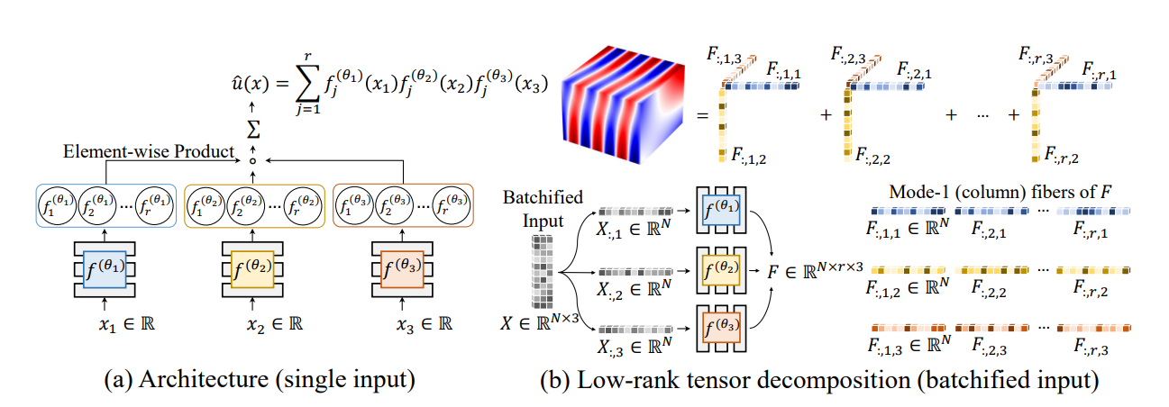
In the Helmholtz problem, each known coordinate point \((x, y, z)\) has a corresponding unknown quantity \(u\) to be solved (here we use \(u\) instead). Here, SPINN is used to represent the mapping function \(f: \mathbb{R}^3 \to \mathbb{R}^1\) from \((x, y, z)\) to \((u)\), that is:

\[ u = m(x, y, z) \]

In the above formula, \(m\) is the SPINN model itself, expressed in PaddleScience code as follows

# set model
model = ppsci.arch.SPINN(**cfg.MODEL)

In order to accurately and quickly access the value of specific variables during calculation, we specify here that the input variable names of the network model are ("x", "y", "z"), and the output variable name is ("u"). These names are consistent with subsequent code.

Then by specifying the number of layers and neurons of SPINN, we instantiate a neural network model model with 4 fully connected layers, each with 64 neurons, and the hidden layer feature dimension r of each output variable is 32, and tanh is used as the activation function.

# model settings
MODEL:
  input_keys: ["x", "y", "z"]
  output_keys: ["u"]
  num_layers: 4
  hidden_size: 64
  r: 32
  activation: "tanh"

3.2 Equation Construction

The Helmholtz differential equation can be represented by the following code:

# set equation
equation = {"Helmholtz": ppsci.equation.Helmholtz(3, 1.0, model)}

Note: Here we need to manually pass the model to equation["Helmholtz"] because the Helmholtz equation needs to use the forward differentiation function.

3.3 Constraint Construction

3.3.1 Interior Point Constraint

Taking SupervisedConstraint acting on interior points as an example, the code for generating interior point training data is as follows:

def _helmholtz3d_exact_u(a1, a2, a3, x, y, z):
    return np.sin(a1 * np.pi * x) * np.sin(a2 * np.pi * y) * np.sin(a3 * np.pi * z)


def _helmholtz3d_source_term(a1, a2, a3, x, y, z, lda=1.0):
    u_gt = _helmholtz3d_exact_u(a1, a2, a3, x, y, z)[..., None]
    uxx = -((a1 * np.pi) ** 2) * u_gt
    uyy = -((a2 * np.pi) ** 2) * u_gt
    uzz = -((a3 * np.pi) ** 2) * u_gt
    return uxx + uyy + uzz + lda * u_gt


def generate_train_helmholtz3d(a1, a2, a3, nc):
    xc = np.random.uniform(-1.0, 1.0, [nc, 1]).astype(dtype)
    yc = np.random.uniform(-1.0, 1.0, [nc, 1]).astype(dtype)
    zc = np.random.uniform(-1.0, 1.0, [nc, 1]).astype(dtype)
    # source term
    xcm, ycm, zcm = np.meshgrid(xc, yc, zc, indexing="ij")
    uc = _helmholtz3d_source_term(a1, a2, a3, xcm, ycm, zcm).astype(dtype)
    # boundary (hard-coded)
    xb = [
        np.asarray([[1.0]], dtype=dtype),
        np.asarray([[-1.0]], dtype=dtype),
        xc,
        xc,
        xc,
        xc,
    ]
    yb = [
        yc,
        yc,
        np.asarray([[1.0]], dtype=dtype),
        np.asarray([[-1.0]], dtype=dtype),
        yc,
        yc,
    ]
    zb = [
        zc,
        zc,
        zc,
        zc,
        np.asarray([[1.0]], dtype=dtype),
        np.asarray([[-1.0]], dtype=dtype),
    ]
    return xc, yc, zc, uc, xb, yb, zb

The code for constructing interior point constraints is as follows:

class InteriorDataGenerator:
    def __init__(self):
        self.iter = 0
        self._gen()

    def _gen(self):
        global xb, yb, zb
        xc, yc, zc, uc, xb, yb, zb = generate_train_helmholtz3d(
            cfg.a1,
            cfg.a2,
            cfg.a3,
            cfg.TRAIN.nc,
        )
        self.xc = xc
        self.yc = yc
        self.zc = zc
        self.uc = uc

    def __call__(self):
        self.iter += 1

        if self.iter % 100 == 0:
            self._gen()

        return {
            "x": self.xc,
            "y": self.yc,
            "z": self.zc,
            "uc": self.uc,
        }

def gen_label_batch(input_batch):
    return {"helmholtz": input_batch["uc"]}

pde_constraint = ppsci.constraint.SupervisedConstraint(
    {
        "dataset": {
            "name": "ContinuousNamedArrayDataset",
            "input": InteriorDataGenerator(),
            "label": gen_label_batch,
        },
    },
    output_expr=equation["Helmholtz"].equations,
    loss=ppsci.loss.MSELoss("mean"),
    name="PDE",
)
# wrap constraints together
constraint = {
    pde_constraint.name: pde_constraint,
}

The first parameter of SupervisedConstraint is the data configuration used for training. Since we use real-time randomly generated data instead of fixed data points, we fill in the custom input data/label generation function;

The second parameter is the equation expression, so pass in the Helmholtz equation object;

The third parameter is the loss function, here MSELoss is selected;

The fourth parameter is the name of the constraint condition. Each constraint condition needs to be named for subsequent indexing. Here it is named "PDE".

3.3.2 Boundary Value Constraint

The third constraint condition is the boundary value constraint, and the code is as follows:

    def __init__(self, idx: int):
        self.idx = idx

    def __call__(self):
        global xb, yb, zb
        tmp = {
            "x": xb[self.idx],
            "y": yb[self.idx],
            "z": zb[self.idx],
        }
        return tmp

def gen_bc_label(data_dict):
    nx = len(data_dict["x"])
    ny = len(data_dict["y"])
    nz = len(data_dict["z"])
    return {"u": np.zeros([nx, ny, nz, 1], dtype=dtype)}

for i in range(6):
    bc_constraint_i = ppsci.constraint.SupervisedConstraint(
        {
            "dataset": {
                "name": "ContinuousNamedArrayDataset",
                "input": BCDataGenerator(i),
                "label": gen_bc_label,
            },
        },
        output_expr={"u": lambda out: out["u"]},
        loss=ppsci.loss.MSELoss("mean"),
        name=f"BC{i}",
    )
    constraint[bc_constraint_i.name] = bc_constraint_i

3.4 Hyperparameter Setting

Next, we need to specify the number of training epochs and learning rate. Here, based on experimental experience, we use 50 training epochs, 1000 steps per epoch, and an initial learning rate of 0.001.

# training settings
TRAIN:
  epochs: 50
  iters_per_epoch: 1000
  save_freq: 10
  eval_during_train: false
  eval_freq: 5
  lr_scheduler:
    epochs: ${TRAIN.epochs}
    iters_per_epoch: ${TRAIN.iters_per_epoch}
    learning_rate: 1.0e-3
    gamma: 0.9
    decay_steps: 1000
    by_epoch: false
  nc: 64
  pretrained_model_path: null
  checkpoint_path: null

3.5 Optimizer Construction

The training process will call the optimizer to update model parameters. Here, the commonly used Adam optimizer is selected, and the ExponentialDecay learning rate adjustment strategy commonly used in machine learning is used together.

lr_scheduler = ppsci.optimizer.lr_scheduler.ExponentialDecay(
    **cfg.TRAIN.lr_scheduler
)()
optimizer = ppsci.optimizer.Adam(lr_scheduler)(model)

3.6 Model Training, Evaluation and Visualization

After completing the above settings, you only need to pass the instantiated objects to ppsci.solver.Solver in order, and then start training, evaluation, and visualization.

solver = ppsci.solver.Solver(
    model,
    constraint,
    optimizer=optimizer,
    equation=equation,
    cfg=cfg,
)
# train model
solver.train()

# evaluate after training
x, y, z, u_gt = generate_test_helmholtz3d(cfg.a1, cfg.a2, cfg.a3, cfg.EVAL.nc)
u_pred = solver.predict(
    {
        "x": x,
        "y": y,
        "z": z,
    },
    batch_size=None,
    return_numpy=True,
)["u"].reshape(-1)
u_gt = u_gt.reshape(-1)
l2_err = np.linalg.norm(u_pred - u_gt, ord=2) / np.linalg.norm(u_gt, ord=2)
rmse = np.sqrt(np.mean((u_pred - u_gt) ** 2))
logger.message(f"l2_err = {l2_err:.4f}, rmse = {rmse:.4f}")

save_result(
    osp.join(cfg.output_dir, "helmholtz3d_result.vtu"), x, y, z, u_pred, u_gt
)

4. Complete Code

"""
Reference: https://github.com/stnamjef/SPINN/blob/main/helmholtz3d.py
"""

from os import path as osp

import hydra
import numpy as np
import paddle
from omegaconf import DictConfig

import ppsci
from ppsci.utils import logger

dtype = paddle.get_default_dtype()


def save_result(filename, x, y, z, u_pred, u_ref):
    xm, ym, zm = np.meshgrid(x, y, z, indexing="ij")
    xm = xm.reshape(-1, 1)
    ym = ym.reshape(-1, 1)
    zm = zm.reshape(-1, 1)
    u_pred = u_pred.reshape(-1, 1)
    u_ref = u_ref.reshape(-1, 1)
    ppsci.visualize.save_vtu_from_dict(
        filename,
        {
            "x": xm,
            "y": ym,
            "z": zm,
            "u_pred": u_pred,
            "u_ref": u_ref,
        },
        ("x", "y", "z"),
        ("u_pred", "u_ref"),
    )


def _helmholtz3d_exact_u(a1, a2, a3, x, y, z):
    return np.sin(a1 * np.pi * x) * np.sin(a2 * np.pi * y) * np.sin(a3 * np.pi * z)


def _helmholtz3d_source_term(a1, a2, a3, x, y, z, lda=1.0):
    u_gt = _helmholtz3d_exact_u(a1, a2, a3, x, y, z)[..., None]
    uxx = -((a1 * np.pi) ** 2) * u_gt
    uyy = -((a2 * np.pi) ** 2) * u_gt
    uzz = -((a3 * np.pi) ** 2) * u_gt
    return uxx + uyy + uzz + lda * u_gt


def generate_train_helmholtz3d(a1, a2, a3, nc):
    xc = np.random.uniform(-1.0, 1.0, [nc, 1]).astype(dtype)
    yc = np.random.uniform(-1.0, 1.0, [nc, 1]).astype(dtype)
    zc = np.random.uniform(-1.0, 1.0, [nc, 1]).astype(dtype)
    # source term
    xcm, ycm, zcm = np.meshgrid(xc, yc, zc, indexing="ij")
    uc = _helmholtz3d_source_term(a1, a2, a3, xcm, ycm, zcm).astype(dtype)
    # boundary (hard-coded)
    xb = [
        np.asarray([[1.0]], dtype=dtype),
        np.asarray([[-1.0]], dtype=dtype),
        xc,
        xc,
        xc,
        xc,
    ]
    yb = [
        yc,
        yc,
        np.asarray([[1.0]], dtype=dtype),
        np.asarray([[-1.0]], dtype=dtype),
        yc,
        yc,
    ]
    zb = [
        zc,
        zc,
        zc,
        zc,
        np.asarray([[1.0]], dtype=dtype),
        np.asarray([[-1.0]], dtype=dtype),
    ]
    return xc, yc, zc, uc, xb, yb, zb


def generate_test_helmholtz3d(a1, a2, a3, nc_test):
    x = np.linspace(-1.0, 1.0, nc_test, dtype=dtype)
    y = np.linspace(-1.0, 1.0, nc_test, dtype=dtype)
    z = np.linspace(-1.0, 1.0, nc_test, dtype=dtype)
    xm, ym, zm = np.meshgrid(x, y, z, indexing="ij")
    u_gt = _helmholtz3d_exact_u(a1, a2, a3, xm, ym, zm).astype(dtype)[..., None]
    x = x.reshape(-1, 1)
    y = y.reshape(-1, 1)
    z = z.reshape(-1, 1)
    return x, y, z, u_gt


def train(cfg: DictConfig):
    # set model
    model = ppsci.arch.SPINN(**cfg.MODEL)

    # set equation
    equation = {"Helmholtz": ppsci.equation.Helmholtz(3, 1.0, model)}

    # set constraint
    class InteriorDataGenerator:
        def __init__(self):
            self.iter = 0
            self._gen()

        def _gen(self):
            global xb, yb, zb
            xc, yc, zc, uc, xb, yb, zb = generate_train_helmholtz3d(
                cfg.a1,
                cfg.a2,
                cfg.a3,
                cfg.TRAIN.nc,
            )
            self.xc = xc
            self.yc = yc
            self.zc = zc
            self.uc = uc

        def __call__(self):
            self.iter += 1

            if self.iter % 100 == 0:
                self._gen()

            return {
                "x": self.xc,
                "y": self.yc,
                "z": self.zc,
                "uc": self.uc,
            }

    def gen_label_batch(input_batch):
        return {"helmholtz": input_batch["uc"]}

    pde_constraint = ppsci.constraint.SupervisedConstraint(
        {
            "dataset": {
                "name": "ContinuousNamedArrayDataset",
                "input": InteriorDataGenerator(),
                "label": gen_label_batch,
            },
        },
        output_expr=equation["Helmholtz"].equations,
        loss=ppsci.loss.MSELoss("mean"),
        name="PDE",
    )
    # wrap constraints together
    constraint = {
        pde_constraint.name: pde_constraint,
    }

    class BCDataGenerator:
        def __init__(self, idx: int):
            self.idx = idx

        def __call__(self):
            global xb, yb, zb
            tmp = {
                "x": xb[self.idx],
                "y": yb[self.idx],
                "z": zb[self.idx],
            }
            return tmp

    def gen_bc_label(data_dict):
        nx = len(data_dict["x"])
        ny = len(data_dict["y"])
        nz = len(data_dict["z"])
        return {"u": np.zeros([nx, ny, nz, 1], dtype=dtype)}

    for i in range(6):
        bc_constraint_i = ppsci.constraint.SupervisedConstraint(
            {
                "dataset": {
                    "name": "ContinuousNamedArrayDataset",
                    "input": BCDataGenerator(i),
                    "label": gen_bc_label,
                },
            },
            output_expr={"u": lambda out: out["u"]},
            loss=ppsci.loss.MSELoss("mean"),
            name=f"BC{i}",
        )
        constraint[bc_constraint_i.name] = bc_constraint_i

    # set optimizer
    lr_scheduler = ppsci.optimizer.lr_scheduler.ExponentialDecay(
        **cfg.TRAIN.lr_scheduler
    )()
    optimizer = ppsci.optimizer.Adam(lr_scheduler)(model)

    # initialize solver
    solver = ppsci.solver.Solver(
        model,
        constraint,
        optimizer=optimizer,
        equation=equation,
        cfg=cfg,
    )
    # train model
    solver.train()

    # evaluate after training
    x, y, z, u_gt = generate_test_helmholtz3d(cfg.a1, cfg.a2, cfg.a3, cfg.EVAL.nc)
    u_pred = solver.predict(
        {
            "x": x,
            "y": y,
            "z": z,
        },
        batch_size=None,
        return_numpy=True,
    )["u"].reshape(-1)
    u_gt = u_gt.reshape(-1)
    l2_err = np.linalg.norm(u_pred - u_gt, ord=2) / np.linalg.norm(u_gt, ord=2)
    rmse = np.sqrt(np.mean((u_pred - u_gt) ** 2))
    logger.message(f"l2_err = {l2_err:.4f}, rmse = {rmse:.4f}")

    save_result(
        osp.join(cfg.output_dir, "helmholtz3d_result.vtu"), x, y, z, u_pred, u_gt
    )


def evaluate(cfg: DictConfig):
    # set model
    model = ppsci.arch.SPINN(**cfg.MODEL)

    solver = ppsci.solver.Solver(
        model,
        cfg=cfg,
    )

    # evaluate
    x, y, z, u_gt = generate_test_helmholtz3d(cfg.a1, cfg.a2, cfg.a3, cfg.EVAL.nc)
    u_pred = solver.predict(
        {
            "x": x,
            "y": y,
            "z": z,
        },
        batch_size=None,
        return_numpy=True,
    )["u"].reshape(-1)
    u_gt = u_gt.reshape(-1)
    l2_err = np.linalg.norm(u_pred - u_gt, ord=2) / np.linalg.norm(u_gt, ord=2)
    rmse = np.sqrt(np.mean((u_pred - u_gt) ** 2))
    logger.message(f"l2_err = {l2_err:.4f}, rmse = {rmse:.4f}")

    save_result(
        osp.join(cfg.output_dir, "helmholtz3d_result.vtu"), x, y, z, u_pred, u_gt
    )


def export(cfg: DictConfig):
    # set model
    model = ppsci.arch.SPINN(**cfg.MODEL)

    # initialize solver
    solver = ppsci.solver.Solver(model, cfg=cfg)
    # export model
    from paddle.static import InputSpec

    input_spec = [
        {key: InputSpec([None, 1], "float32", name=key) for key in model.input_keys},
    ]
    solver.export(input_spec, cfg.INFER.export_path, with_onnx=False)


def inference(cfg: DictConfig):
    from deploy.python_infer import pinn_predictor

    predictor = pinn_predictor.PINNPredictor(cfg)

    # evaluate
    x, y, z, u_gt = generate_test_helmholtz3d(cfg.a1, cfg.a2, cfg.a3, cfg.EVAL.nc)
    output_dict = predictor.predict(
        {
            "x": x,
            "y": y,
            "z": z,
        },
        batch_size=None,
    )
    # mapping data to cfg.INFER.output_keys
    output_dict = {
        store_key: output_dict[infer_key]
        for store_key, infer_key in zip(cfg.MODEL.output_keys, output_dict.keys())
    }
    u_pred = output_dict["u"].reshape(-1)
    u_gt = u_gt.reshape(-1)
    l2_err = np.linalg.norm(u_pred - u_gt, ord=2) / np.linalg.norm(u_gt, ord=2)
    rmse = np.sqrt(np.mean((u_pred - u_gt) ** 2))
    logger.message(f"l2_err = {l2_err:.4f}, rmse = {rmse:.4f}")

    save_result(
        osp.join(cfg.output_dir, "helmholtz3d_result.vtu"), x, y, z, u_pred, u_gt
    )


@hydra.main(version_base=None, config_path="./conf", config_name="helmholtz3d.yaml")
def main(cfg: DictConfig):
    if cfg.mode == "train":
        train(cfg)
    elif cfg.mode == "eval":
        evaluate(cfg)
    elif cfg.mode == "export":
        export(cfg)
    elif cfg.mode == "infer":
        inference(cfg)
    else:
        raise ValueError(
            f"cfg.mode should in ['train', 'eval', 'export', 'infer'], but got '{cfg.mode}'"
        )


if __name__ == "__main__":
    main()

5. Result Display

Sample \(100^3\) points uniformly on the computational domain, and their prediction results and analytical solutions are shown in the figure below.

Left is PaddleScience prediction result, right is analytical solution result

The error predicted by the model in this problem is l2_err = 0.0183, rmse = 0.0064, which is small and basically consistent with the analytical solution error.

6. References

• Separable Physics-Informed Neural Networks
• SPINN