Skip to content

Bubble_flow

# linux
wget -c https://paddle-org.bj.bcebos.com/paddlescience/datasets/BubbleNet/bubble.mat
# windows
# curl https://paddle-org.bj.bcebos.com/paddlescience/datasets/BubbleNet/bubble.mat -o bubble.mat
python bubble.py
# linux
wget -c https://paddle-org.bj.bcebos.com/paddlescience/datasets/BubbleNet/bubble.mat
# windows
# curl https://paddle-org.bj.bcebos.com/paddlescience/datasets/BubbleNet/bubble.mat -o bubble.mat
python bubble.py mode=eval EVAL.pretrained_model_path=https://paddle-org.bj.bcebos.com/paddlescience/models/bubble/bubble_pretrained.pdparams
python bubble.py mode=export
# linux
wget -c https://paddle-org.bj.bcebos.com/paddlescience/datasets/BubbleNet/bubble.mat
# windows
# curl https://paddle-org.bj.bcebos.com/paddlescience/datasets/BubbleNet/bubble.mat -o bubble.mat
python bubble.py mode=infer
Pretrained Model Metrics
bubble_pretrained.pdparams loss(bubble_mse): 0.00558
MSE.u(bubble_mse): 0.00090
MSE.v(bubble_mse): 0.00322
MSE.p(bubble_mse): 0.00066
MSE.phil(bubble_mse): 0.00079

1. Background Introduction

1.1 Bubble Flow

Bubble flow is a typical representative of multiphase flow. Multiphase flow studies the common scientific problems in multiphase fluid dynamics, thermodynamics, heat and mass transfer, combustion, chemical and biological reactions, and related industrial processes where two or more substances of different phases or components coexist with clear interfaces. This is an emerging interdisciplinary science that has gradually developed from the field of traditional energy conversion and utilization, involving many fields such as energy, power, nuclear reactors, chemical engineering, petroleum, refrigeration, cryogenics, renewable energy development and utilization, aerospace, environmental protection, life sciences, etc., and plays an irreplaceable huge role in the development of basic and pillar industries of the national economy and national defense science and technology. In multiphase flow, there are obvious interfaces between phases, and each maintains relatively independent material properties, such as gas-liquid, gas-solid, liquid-liquid, liquid-solid, etc. In this article, we mainly study bubble flow. Of course, some semi-physics-informed neural networks (Semi-PINNs) methods introduced in this article are also applicable to multiphase flow problems.

Bubble flow is a fluid mechanics phenomenon that occurs when a gas-liquid two-phase mixture flows in a tube under the action of force and the gas content in the mixture is low. At this time, the gas phase is distributed in the liquid phase as dispersed small bubbles. There are more bubbles in the center of the tube and fewer bubbles near the tube wall. These small bubbles are approximately spherical, and their moving speed is greater than the liquid flow speed. This flow pattern is called bubble flow. Bubble flow has been widely used in various fields, such as

  • Chemical processes: In chemical processes, bubble flow often occurs where there is a large amount of gas in the liquid, such as in gas absorption, desorption, extraction, emulsification, etc. The characteristics of bubble flow have an important impact on the optimization of process flow and the selection of equipment.
  • Biomedicine: In the field of biomedicine, bubble flow is often used for drug delivery, cell separation, bioreactor design, etc. For example, by controlling the size and flow rate of bubbles, drugs can be accurately delivered to the target site.
  • Environmental engineering: In environmental engineering, bubble flow can be used in water treatment, wastewater treatment, gas purification, etc. For example, oxygen can be introduced into sewage through bubble flow to promote the growth of microorganisms, thereby accelerating the decomposition of organic waste.
  • Food industry: In the food industry, bubble flow also has a wide range of applications. For example, when making bread, cakes and other foods, the fermentation process of the dough can be controlled through the characteristics of bubble flow to obtain better taste and texture.
  • Aerospace: In the field of aerospace, the study of bubble flow can help designers better understand the flow characteristics of complex fluid dynamic systems such as aircraft and rockets, thereby optimizing design and improving performance.
  • Petroleum industry: In the petroleum industry, bubble flow often appears in oil production, oil transportation, refining and other processes. Bubble flow can increase the tension of the oil-water interface and improve oil recovery efficiency.

The research and application of bubble flow are of great significance to many fields. It not only helps us deeply understand the basic principles of fluid dynamics, but also provides useful guidance and help for actual production and engineering applications. At the same time, because bubble flow is a classic fluid mechanics problem with high density gradients, it is often used to test the effectiveness of algorithms.

1.2 Semi-PINNs Method

Physics-informed Neural Networks (PINNs) are physical models based on neural networks designed to solve supervised learning tasks while respecting physical laws described by nonlinear partial differential equations. This network not only learns the distribution rules of training data samples, but also learns the physical laws described by mathematical equations.

The background of PINNs stems from the combination of data-driven methods and physical models. In many scientific and engineering applications, due to the high difficulty and complexity of collecting training data, pure data-driven methods often fail to achieve ideal results. At the same time, although traditional physical models can accurately describe natural phenomena, they may not be able to fully utilize all available data in some cases. Therefore, as a method combining data-driven and physical models, PINN aims to leverage the advantages of both to improve prediction accuracy and generalization ability.

The principle of PINNs is to use physical equations as regularizers and neural networks as solvers, compare the results predicted by neural networks with actual observation data, and update the weights of neural networks through back-propagation algorithms to reduce prediction errors. This method considers physical constraints during training, so it can more accurately capture the dynamic behavior of the system.

Although PINN has many advantages, such as being able to handle high-dimensional data and solve inverse problems, it still has some limitations. For example, the consideration of physical equations in the loss function usually requires high-order differentiation of physical quantities. Especially in two-phase flow, the phase value at the interface of different fluids shows a drastic change from 0 to 1, making the calculation of gradients very difficult. Therefore, for variables with high gradients, high-resolution training data will be a prerequisite for the success of the algorithm, but this will greatly increase the computational cost of deep learning, and it is also difficult to obtain high-resolution data in many experiments.

To this end, we do not use complete fluid dynamic equations to supervise the training process of bubble flow, but based on partial physical information to obtain satisfactory results. Specifically, we only substitute the fluid continuity condition (\(\nabla \mathbf{u} =0\)) and the pressure Poisson equation (denoted as \(\mathcal{P}\)) into the loss function, which can be described as a neural network with partial physical information - Semi-PINNs.

2. Problem Definition

2.1 Bubble Flow Governing Equations

The bubble flow model is generally described by the Navier–Stokes equations,

\[ \begin{cases} \begin{aligned} &\nabla \cdot \mathbf{u}=0, \\ &\rho\left(\frac{\partial \mathbf{u}}{\partial t}+(\mathbf{u} \cdot \nabla) \mathbf{u}\right)=-\nabla p+\mu \nabla^2 \mathbf{u}, \end{aligned} \end{cases} \]

where \(\rho\) is the fluid density, \(\mathbf{u} = ( u , v )\) is the two-dimensional velocity vector, \(p\) is the fluid pressure, and \(\mu\) is the dynamic viscosity. The interface between air and water is represented by the contour line of a certain level set or globally defined function, that is, defining the level set function \(\phi = \phi ( x , y , t )\) in two-dimensional space. For water \(\phi=0\), for air \(\phi=1\). Near the interface between the two, there is a smooth transition from 0 to 1, and the level set of the interface is set to \(\phi= 0.5\).

Let \(\rho_l\) be the water (liquid) density, \(\rho_g\) be the air (gas) density, \(\mu_l\) be the water viscosity, and \(\mu_g\) be the air viscosity, then the density and viscosity in the fluid can be expressed by the level set function as:

\[\begin{aligned} \rho & =\rho_l+\phi\left(\rho_g-\rho_l\right), \\ \mu & =\mu_l+\phi\left(\mu_g-\mu_l\right) . \end{aligned}\]

To simulate the interface between liquid and gas, the level set function \(\phi = \phi ( x , y , t )\) is defined as

\[\frac{\partial \phi}{\partial t}+\mathbf{u} \cdot \nabla \phi=\gamma \nabla \cdot\left(\epsilon_{l s} \nabla \phi-\phi(1-\phi) \frac{\nabla \phi}{|\nabla \phi|}\right),\]

where the left side of the equal sign describes the movement of the interface, while the right side aims to keep the interface compact and numerically stable. \(\gamma\) is the initialization parameter, which determines the re-initialization or stabilization amount of the level set function, and \(\epsilon_{l s}\) is the parameter controlling the interface thickness, which is equal to the maximum grid size.

2.2 BubbleNet (Semi-PINNs Method)

The study of bubble flow problems can usually be divided into single bubble flow (Figure A) and multi-bubble flow (Figure B).

bubble.png

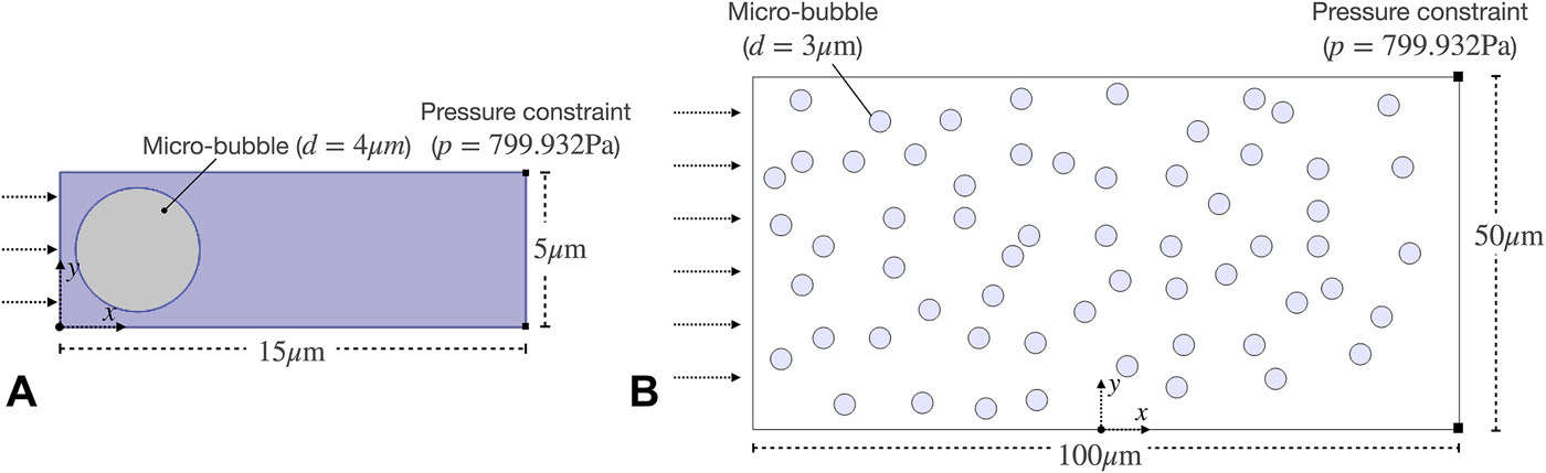
In this article, we mainly consider single bubble flow (Figure A), which is of course also applicable to multi-bubble flow problems. For the single bubble case, the initial bubble diameter is set to \(d = 4~μm\), the microchannel length is \(15~μm\), and the width is \(5~μm\). A pressure difference \(\Delta p = 10~Pa\) is applied along the axial direction to drive the bubble flow, and the pressure at the end of the channel is maintained at a constant pressure \(p_0 = 799.932~Pa(6~mmHg)\), corresponding to the pressure of interstitial fluid in the human brain and lymphatic flow. The initial condition (IC) is set to \(p=p_0\) and the room temperature is \(293.15~K\), as shown in Figure A. This numerical setting aims to simulate bubble transport in cerebral blood vessels to study the blood-brain barrier. At the same time, we set \(\gamma=1\) and \(\epsilon_{l s}=0.430\).

The main content of the BubbleNet algorithm in this article is as follows:

  • Use Time Discrete Normalization (TDN), that is
\[\mathcal{W}=\frac{\mathcal{U}-\mathcal{U}_{\min }}{\mathcal{U}_{\max }-\mathcal{U}_{\min }},\]

where \(\mathcal{U}=(u, v, p, \phi)\) is the coarsened data obtained from the bubble flow simulation, and \(\mathcal{U}_{\min },~\mathcal{U}_{\max }\) are the maximum and minimum values of the coarsened CFD data at each time step, respectively. The reason for this processing is that the physical quantities in the flow field vary greatly, and TDN will help eliminate inaccuracies caused by changes in physical quantities.

  • Introduce the stream function \(\psi\) to predict the velocity fields \(u\), \(v\), that is
\[u=\frac{\partial \psi}{\partial y},\quad v=-\frac{\partial \psi}{\partial x},\]

The introduction of the stream function avoids the gradient calculation of the velocity vector in the loss function and improves the efficiency of the neural network.

  • Introduce the pressure Poisson equation to improve the accuracy of prediction, that is, take the divergence of both ends of the momentum equation simultaneously:
\[\nabla^2 p=\rho \frac{\nabla \cdot \mathbf{u}}{\Delta t}-\rho \nabla \cdot(\mathbf{u} \cdot \nabla \mathbf{u})+\mu \nabla^2(\nabla \cdot \mathbf{u}) = -\rho \nabla \cdot(\mathbf{u} \cdot \nabla \mathbf{u}).\]
  • Use Mean Squared Error (MSE) to calculate the deviation between predicted and training data in the loss function. The loss function is expressed as
\[\mathcal{L}=\frac{1}{m} \sum_{i=1}^m\left(\mathcal{W}_{\text {pred }(i)}-\mathcal{W}_{\text {train }(i)}\right)^2+\frac{1}{m} \sum_{i=1}^m\left(\nabla^2 p_{(i)}\right)^2,\]

where \(\mathcal{W}=(u, v, p, \phi)\) represents the normalized dataset.

For the single bubble flow problem, the model structure diagram of BubbleNet (Semi-PINNs method) proposed in this article is:

pinns.jpeg

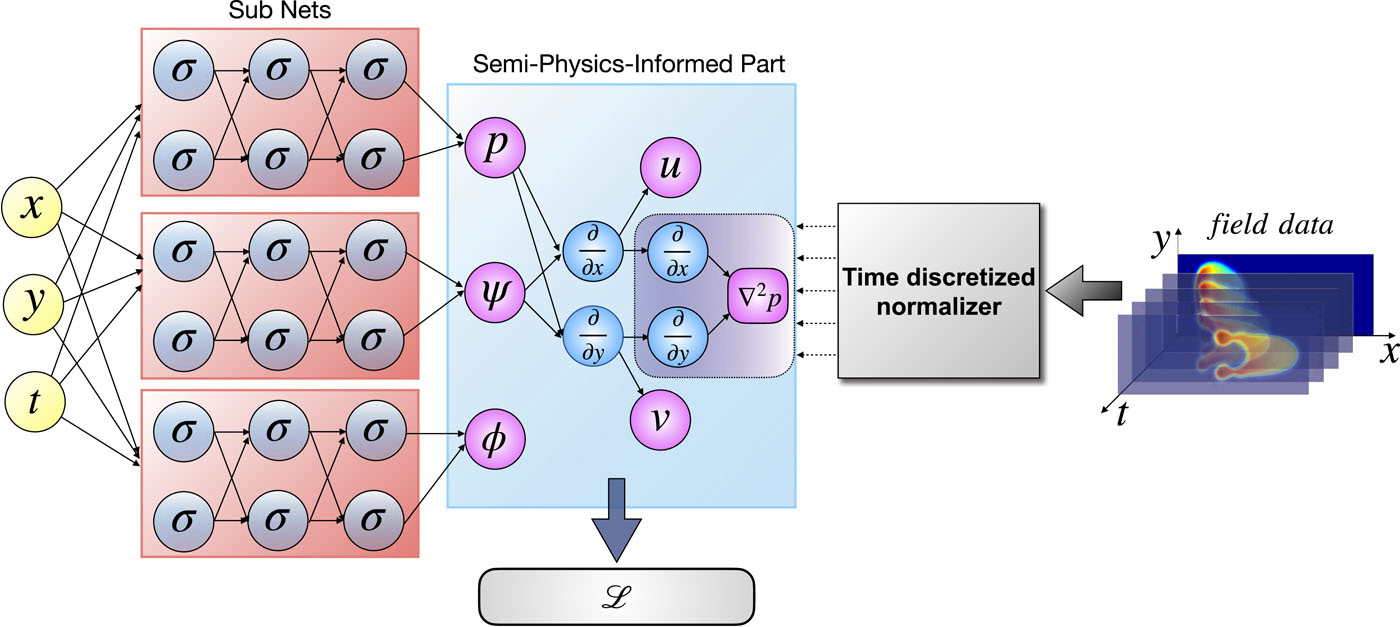
Here we use three subnets: \(Net_{\psi},~Net_p\) and \(Net_{\phi}\) to predict \(\psi\), \(p\) and \(\phi\) respectively, and calculate velocity \(u,~v\) by automatic differentiation of \(\psi\).

3. Problem Solving

Next, we will explain how to convert the problem into PaddleScience code step by step and solve the single bubble flow problem using deep learning methods. In order to quickly understand PaddleScience, only key steps such as model construction and constraint construction are described below, while other details please refer to API Documentation.

3.1 Data Processing

The dataset is obtained from CFD results under fine grids, containing unnormalized \(x,~y,~t,~u,~v,~p,~\phi\), stored in the form of a dictionary in a .mat file. Before running the code for this problem, please download the dataset.

After downloading, we first need to perform Time Discrete Normalization (TDN) on the dataset, and construct the training set and validation set.

# load Data
data = scipy.io.loadmat(cfg.DATA_PATH)
# normalize data
p_max = data["p"].max(axis=0)
p_min = data["p"].min(axis=0)
p_norm = (data["p"] - p_min) / (p_max - p_min)
u_max = data["u"].max(axis=0)
u_min = data["u"].min(axis=0)
u_norm = (data["u"] - u_min) / (u_max - u_min)
v_max = data["v"].max(axis=0)
v_min = data["v"].min(axis=0)
v_norm = (data["v"] - v_min) / (v_max - v_min)

u_star = u_norm  # N x T
v_star = v_norm  # N x T
p_star = p_norm  # N x T
phil_star = data["phil"]  # N x T
t_star = data["t"]  # T x 1
x_star = data["X"]  # N x 2

N = x_star.shape[0]
T = t_star.shape[0]

# rearrange data
xx = np.tile(x_star[:, 0:1], (1, T))  # N x T
yy = np.tile(x_star[:, 1:2], (1, T))  # N x T
tt = np.tile(t_star, (1, N)).T  # N x T

x = xx.flatten()[:, None].astype(paddle.get_default_dtype())  # NT x 1
y = yy.flatten()[:, None].astype(paddle.get_default_dtype())  # NT x 1
t = tt.flatten()[:, None].astype(paddle.get_default_dtype())  # NT x 1

u = u_star.flatten()[:, None].astype(paddle.get_default_dtype())  # NT x 1
v = v_star.flatten()[:, None].astype(paddle.get_default_dtype())  # NT x 1
p = p_star.flatten()[:, None].astype(paddle.get_default_dtype())  # NT x 1
phil = phil_star.flatten()[:, None].astype(paddle.get_default_dtype())  # NT x 1

idx = np.random.choice(N * T, int(N * T * 0.75), replace=False)
# train data
train_input = {"x": x[idx, :], "y": y[idx, :], "t": t[idx, :]}
train_label = {"u": u[idx, :], "v": v[idx, :], "p": p[idx, :], "phil": phil[idx, :]}

# eval data
test_input = {"x": x, "y": y, "t": t}
test_label = {"u": u, "v": v, "p": p, "phil": phil}

3.2 Model Construction

In the bubble flow problem, each known coordinate point \((t, x, y)\) has three unknown quantities to be solved: stream function \(\psi\), pressure \(p\) and level set function \(\phi\). Here we use 3 parallel MLPs (Multilayer Perceptron) to represent the mapping functions \(f_i: \mathbb{R}^3 \to \mathbb{R}\) from \((t, x, y)\) to \((\psi, p, \phi)\) respectively, that is:

\[ \begin{aligned} \psi &= f_1(t, x, y),\\ p &= f_2(t, x, y),\\ \phi &= f_3(t, x, y). \end{aligned} \]

In the above formula, \(f_1,f_2,f_3\) are all MLP models, expressed in PaddleScience code as follows

# set model
model_psi = ppsci.arch.MLP(**cfg.MODEL.psi_net)
model_p = ppsci.arch.MLP(**cfg.MODEL.p_net)
model_phil = ppsci.arch.MLP(**cfg.MODEL.phil_net)

Use transform_out function to implement the transformation from stream function \(\psi\) to velocity \(u,~v\), the code is as follows

# transform
def transform_out(in_, out):
    psi_y = out["psi"]
    y = in_["y"]
    x = in_["x"]
    u = jacobian(psi_y, y)
    v = -jacobian(psi_y, x)
    return {"u": u, "v": v}

At the same time, the corresponding transform needs to be registered for the model model_psi, and then the 3 MLP models are composed into Model_List

# register transform
model_psi.register_output_transform(transform_out)
model_list = ppsci.arch.ModelList((model_psi, model_p, model_phil))

In this way, we instantiated a neural network model model_list with 3 MLP models, each MLP containing 9 hidden layers, 30 neurons per layer, using "tanh" as the activation function, and containing output transform.

3.3 Computational Domain Construction

The training area of the single bubble flow in this article is composed of point clouds stored in the dictionary train_input, so you can directly use the point cloud geometry PointCloud built in PaddleScience to read in data and combine it into a time-space computational domain.

At the same time, construct a visualization area, that is, a two-dimensional rectangular area with [0, 0], [15, 5] as the diagonal, and the time domain is 126 moments [1, 2,..., 125, 126]. This area can directly use the spatial geometry Rectangle and time domain TimeDomain built in PaddleScience, combined into a time-space TimeXGeometry computational domain. The code is as follows

# set time-geometry
# set timestamps(including initial t0)
timestamps = np.linspace(0, 126, 127, endpoint=True)
geom = {
    "time_rect": ppsci.geometry.PointCloud(
        train_input,
        ("t", "x", "y"),
    ),
    "time_rect_visu": ppsci.geometry.TimeXGeometry(
        ppsci.geometry.TimeDomain(1, 126, timestamps=timestamps),
        ppsci.geometry.Rectangle((0, 0), (15, 5)),
    ),
}
Tip

Rectangle and TimeDomain are two Geometry derived classes that can be used independently.

If the input data only comes from a two-dimensional rectangular geometric domain, you can directly use ppsci.geometry.Rectangle(...) to create a spatial geometric domain object;

If the input data only comes from a one-dimensional time domain, you can directly use ppsci.geometry.TimeDomain(...) to construct a time domain object.

3.4 Constraint Construction

According to the loss function expression defined in 2.2 BubbleNet (Semi-PINNs Method), corresponding to the two constraints guiding model training in the computational domain, next use the InteriorConstraint and SupervisedConstraint built in PaddleScience to construct the above two constraints.

3.4.1 Interior Point Constraint

We use the interior point constraint InteriorConstraint to implement the constraint of adding the pressure Poisson equation to the loss function. The code is as follows:

# set constraint
pde_constraint = ppsci.constraint.InteriorConstraint(
    {
        "pressure_Poisson": lambda out: hessian(out["p"], out["x"])
        + hessian(out["p"], out["y"])
    },
    {"pressure_Poisson": 0},
    geom["time_rect"],
    {
        "dataset": "IterableNamedArrayDataset",
        "batch_size": cfg.TRAIN.batch_size.pde_constraint,
        "iters_per_epoch": cfg.TRAIN.iters_per_epoch,
    },
    ppsci.loss.MSELoss("mean"),
    name="EQ",
)

The first parameter of InteriorConstraint is the equation expression, used to calculate the equation result, here calculate \(\nabla^2 p_{(i)}\) in the second term of the loss function expression;

The second parameter is the target value of the constraint variable. In this problem, we hope that the result of \(\nabla^2 p_{(i)}\) is optimized to 0, so set the target value to 0;

The third parameter is the computational domain on which the constraint equation acts. Here, fill in geom["time_rect"] instantiated in the 3.3 Computational Domain Construction chapter;

The fourth parameter is the sampling configuration on the computational domain. Here we use full data points for training, so the dataset field is set to "IterableNamedArrayDataset" and iters_per_epoch is also set to 1, and the sampling point number batch_size is set to 228595;

The fifth parameter is the loss function. Here we choose the commonly used MSE function, and reduction is set to "mean", that is, we will calculate the average value of the loss terms generated by all data points involved in the calculation;

The sixth parameter is the name of the constraint condition. We need to name each constraint condition for subsequent indexing. Here we name it "EQ".

3.4.2 Supervised Constraint

At the same time, training is performed in a supervised learning manner on the training data. Here, the supervised constraint SupervisedConstraint is adopted:

sup_constraint = ppsci.constraint.SupervisedConstraint(
    {
        "dataset": {
            "name": "NamedArrayDataset",
            "input": train_input,
            "label": train_label,
        },
        "batch_size": cfg.TRAIN.batch_size.sup_constraint,
        "sampler": {
            "name": "BatchSampler",
            "drop_last": False,
            "shuffle": True,
        },
    },
    ppsci.loss.MSELoss("mean"),
    name="Sup",
)

The first parameter of SupervisedConstraint is the reading configuration of the supervised constraint, where the "dataset" field represents the training dataset information used, and each field represents:

  1. name: Dataset type, here "NamedArrayDataset" means dataset of .mat type read sequentially in batches;
  2. input_keys: Input variable names;
  3. label_keys: Label variable names.

The "sampler" field defines the Sampler class name used as BatchSampler, and also specifies that the parameters drop_last is False and shuffle is True during initialization of this class.

The second parameter is the loss function. Here we choose the commonly used MSE function, and reduction is "mean", that is, we will sum and average the loss terms generated by all data points involved in the calculation;

The third parameter is the name of the constraint condition. We need to name each constraint condition for subsequent indexing. Here we name it "Sup".

After the differential equation constraint and supervised constraint are constructed, encapsulate them into a dictionary with the names we just named as keys for subsequent access.

# wrap constraints together
constraint = {
    sup_constraint.name: sup_constraint,
    pde_constraint.name: pde_constraint,
}

3.5 Hyperparameter Setting

Next, we need to specify the number of training epochs and learning rate. Here, based on experimental experience, we use 10,000 training epochs, evaluation interval is 1,000 epochs, and learning rate is set to 0.001.

# training settings
TRAIN:
  epochs: 10000
  iters_per_epoch: 1
  eval_during_train: true

3.6 Optimizer Construction

The training process will call the optimizer to update model parameters. Here, the more commonly used Adam optimizer is selected.

# set optimizer
optimizer = ppsci.optimizer.Adam(cfg.TRAIN.learning_rate)(model_list)

3.7 Validator Construction

Usually during the training process, the training status of the current model is evaluated using the validation set (test set) at a certain epoch interval, so ppsci.validate.SupervisedValidator is used to construct the validator.

# set validator
mse_validator = ppsci.validate.SupervisedValidator(
    {
        "dataset": {
            "name": "NamedArrayDataset",
            "input": test_input,
            "label": test_label,
        },
        "batch_size": cfg.TRAIN.batch_size.mse_validator,
        "sampler": {
            "name": "BatchSampler",
            "drop_last": False,
            "shuffle": False,
        },
    },
    ppsci.loss.MSELoss("mean"),
    metric={"MSE": ppsci.metric.MSE()},
    name="bubble_mse",
)
validator = {
    mse_validator.name: mse_validator,
}

The configuration is similar to the setting of 3.4 Constraint Construction.

3.8 Model Training and Evaluation

After completing the above settings, you only need to pass the instantiated objects to ppsci.solver.Solver in order, and then start training and evaluation.

solver = ppsci.solver.Solver(
    model_list,
    constraint,
    cfg.output_dir,
    optimizer,
    None,
    cfg.TRAIN.epochs,
    cfg.TRAIN.iters_per_epoch,
    eval_during_train=cfg.TRAIN.eval_during_train,
    eval_freq=cfg.TRAIN.eval_freq,
    geom=geom,
    validator=validator,
)
# train model
solver.train()
# evaluate after finished training
solver.eval()

3.9 Result Visualization

Finally, prediction and visualization are performed on the given visualization area. The visualization data is a two-dimensional point set in the area. The coordinates of each moment \(t\) are \((x^t_i, y^t_i)\), and the corresponding value is \((u^t_i, v^t_i, p^t_i,\phi^t_i)\). Here we denormalize the predicted \((u^t_i, v^t_i, p^t_i,\phi^t_i)\). We save the denormalized data as 126 vtu format files according to time, and finally open them with visualization software to view. The code is as follows:

pred_norm = solver.predict(visu_mat, None, 4096, no_grad=False, return_numpy=True)
# inverse normalization
p_pred = pred_norm["p"].reshape([NTIME_PDE, NPOINT_PDE]).T
u_pred = pred_norm["u"].reshape([NTIME_PDE, NPOINT_PDE]).T
v_pred = pred_norm["v"].reshape([NTIME_PDE, NPOINT_PDE]).T
pred = {
    "p": (p_pred * (p_max - p_min) + p_min).T.reshape([-1, 1]),
    "u": (u_pred * (u_max - u_min) + u_min).T.reshape([-1, 1]),
    "v": (v_pred * (v_max - v_min) + v_min).T.reshape([-1, 1]),
    "phil": pred_norm["phil"],
}
logger.message("Now saving visual result to: visual/result.vtu, please wait...")
ppsci.visualize.save_vtu_from_dict(
    osp.join(cfg.output_dir, "visual/result.vtu"),
    {
        "t": visu_mat["t"],
        "x": visu_mat["x"],
        "y": visu_mat["y"],
        "u": pred["u"],
        "v": pred["v"],
        "p": pred["p"],
        "phil": pred["phil"],
    },
    ("t", "x", "y"),
    ("u", "v", "p", "phil"),
    NTIME_PDE,
)

4. Complete Code

bubble.py
  1
  2
  3
  4
  5
  6
  7
  8
  9
 10
 11
 12
 13
 14
 15
 16
 17
 18
 19
 20
 21
 22
 23
 24
 25
 26
 27
 28
 29
 30
 31
 32
 33
 34
 35
 36
 37
 38
 39
 40
 41
 42
 43
 44
 45
 46
 47
 48
 49
 50
 51
 52
 53
 54
 55
 56
 57
 58
 59
 60
 61
 62
 63
 64
 65
 66
 67
 68
 69
 70
 71
 72
 73
 74
 75
 76
 77
 78
 79
 80
 81
 82
 83
 84
 85
 86
 87
 88
 89
 90
 91
 92
 93
 94
 95
 96
 97
 98
 99
100
101
102
103
104
105
106
107
108
109
110
111
112
113
114
115
116
117
118
119
120
121
122
123
124
125
126
127
128
129
130
131
132
133
134
135
136
137
138
139
140
141
142
143
144
145
146
147
148
149
150
151
152
153
154
155
156
157
158
159
160
161
162
163
164
165
166
167
168
169
170
171
172
173
174
175
176
177
178
179
180
181
182
183
184
185
186
187
188
189
190
191
192
193
194
195
196
197
198
199
200
201
202
203
204
205
206
207
208
209
210
211
212
213
214
215
216
217
218
219
220
221
222
223
224
225
226
227
228
229
230
231
232
233
234
235
236
237
238
239
240
241
242
243
244
245
246
247
248
249
250
251
252
253
254
255
256
257
258
259
260
261
262
263
264
265
266
267
268
269
270
271
272
273
274
275
276
277
278
279
280
281
282
283
284
285
286
287
288
289
290
291
292
293
294
295
296
297
298
299
300
301
302
303
304
305
306
307
308
309
310
311
312
313
314
315
316
317
318
319
320
321
322
323
324
325
326
327
328
329
330
331
332
333
334
335
336
337
338
339
340
341
342
343
344
345
346
347
348
349
350
351
352
353
354
355
356
357
358
359
360
361
362
363
364
365
366
367
368
369
370
371
372
373
374
375
376
377
378
379
380
381
382
383
384
385
386
387
388
389
390
391
392
393
394
395
396
397
398
399
400
401
402
403
404
405
406
407
408
409
410
411
412
413
414
415
416
417
418
419
420
421
422
423
424
425
426
427
428
429
430
431
432
433
434
435
436
437
438
439
440
441
442
443
444
445
446
447
448
449
450
451
452
453
454
455
456
457
458
459
460
461
462
463
464
465
466
467
468
469
470
471
472
473
474
475
476
477
478
479
480
481
482
483
484
485
486
487
488
489
490
491
492
493
494
495
496
497
498
499
500
501
502
503
504
505
506
507
508
509
510
511
512
513
514
515
516
517
518
519
520
521
# Copyright (c) 2023 PaddlePaddle Authors. All Rights Reserved.

# Licensed under the Apache License, Version 2.0 (the "License");
# you may not use this file except in compliance with the License.
# You may obtain a copy of the License at

#     http://www.apache.org/licenses/LICENSE-2.0

# Unless required by applicable law or agreed to in writing, software
# distributed under the License is distributed on an "AS IS" BASIS,
# WITHOUT WARRANTIES OR CONDITIONS OF ANY KIND, either express or implied.
# See the License for the specific language governing permissions and
# limitations under the License.

"""
Reference: https://github.com/hanfengzhai/BubbleNet
Bubble data files download link: https://paddle-org.bj.bcebos.com/paddlescience/datasets/BubbleNet/bubble.mat
"""

from os import path as osp

import hydra
import numpy as np
import paddle
import scipy
from omegaconf import DictConfig

import ppsci
from ppsci.autodiff import hessian
from ppsci.autodiff import jacobian
from ppsci.utils import logger


def train(cfg: DictConfig):
    # set random seed for reproducibility
    ppsci.utils.misc.set_random_seed(cfg.seed)
    # initialize logger
    logger.init_logger("ppsci", osp.join(cfg.output_dir, f"{cfg.mode}.log"), "info")

    # load Data
    data = scipy.io.loadmat(cfg.DATA_PATH)
    # normalize data
    p_max = data["p"].max(axis=0)
    p_min = data["p"].min(axis=0)
    p_norm = (data["p"] - p_min) / (p_max - p_min)
    u_max = data["u"].max(axis=0)
    u_min = data["u"].min(axis=0)
    u_norm = (data["u"] - u_min) / (u_max - u_min)
    v_max = data["v"].max(axis=0)
    v_min = data["v"].min(axis=0)
    v_norm = (data["v"] - v_min) / (v_max - v_min)

    u_star = u_norm  # N x T
    v_star = v_norm  # N x T
    p_star = p_norm  # N x T
    phil_star = data["phil"]  # N x T
    t_star = data["t"]  # T x 1
    x_star = data["X"]  # N x 2

    N = x_star.shape[0]
    T = t_star.shape[0]

    # rearrange data
    xx = np.tile(x_star[:, 0:1], (1, T))  # N x T
    yy = np.tile(x_star[:, 1:2], (1, T))  # N x T
    tt = np.tile(t_star, (1, N)).T  # N x T

    x = xx.flatten()[:, None].astype(paddle.get_default_dtype())  # NT x 1
    y = yy.flatten()[:, None].astype(paddle.get_default_dtype())  # NT x 1
    t = tt.flatten()[:, None].astype(paddle.get_default_dtype())  # NT x 1

    u = u_star.flatten()[:, None].astype(paddle.get_default_dtype())  # NT x 1
    v = v_star.flatten()[:, None].astype(paddle.get_default_dtype())  # NT x 1
    p = p_star.flatten()[:, None].astype(paddle.get_default_dtype())  # NT x 1
    phil = phil_star.flatten()[:, None].astype(paddle.get_default_dtype())  # NT x 1

    idx = np.random.choice(N * T, int(N * T * 0.75), replace=False)
    # train data
    train_input = {"x": x[idx, :], "y": y[idx, :], "t": t[idx, :]}
    train_label = {"u": u[idx, :], "v": v[idx, :], "p": p[idx, :], "phil": phil[idx, :]}

    # eval data
    test_input = {"x": x, "y": y, "t": t}
    test_label = {"u": u, "v": v, "p": p, "phil": phil}

    # set model
    model_psi = ppsci.arch.MLP(**cfg.MODEL.psi_net)
    model_p = ppsci.arch.MLP(**cfg.MODEL.p_net)
    model_phil = ppsci.arch.MLP(**cfg.MODEL.phil_net)

    # transform
    def transform_out(in_, out):
        psi_y = out["psi"]
        y = in_["y"]
        x = in_["x"]
        u = jacobian(psi_y, y)
        v = -jacobian(psi_y, x)
        return {"u": u, "v": v}

    # register transform
    model_psi.register_output_transform(transform_out)
    model_list = ppsci.arch.ModelList((model_psi, model_p, model_phil))

    # set time-geometry
    # set timestamps(including initial t0)
    timestamps = np.linspace(0, 126, 127, endpoint=True)
    geom = {
        "time_rect": ppsci.geometry.PointCloud(
            train_input,
            ("t", "x", "y"),
        ),
        "time_rect_visu": ppsci.geometry.TimeXGeometry(
            ppsci.geometry.TimeDomain(1, 126, timestamps=timestamps),
            ppsci.geometry.Rectangle((0, 0), (15, 5)),
        ),
    }

    NTIME_ALL = len(timestamps)
    NPOINT_PDE, NTIME_PDE = 300 * 100, NTIME_ALL - 1

    # set constraint
    pde_constraint = ppsci.constraint.InteriorConstraint(
        {
            "pressure_Poisson": lambda out: hessian(out["p"], out["x"])
            + hessian(out["p"], out["y"])
        },
        {"pressure_Poisson": 0},
        geom["time_rect"],
        {
            "dataset": "IterableNamedArrayDataset",
            "batch_size": cfg.TRAIN.batch_size.pde_constraint,
            "iters_per_epoch": cfg.TRAIN.iters_per_epoch,
        },
        ppsci.loss.MSELoss("mean"),
        name="EQ",
    )

    sup_constraint = ppsci.constraint.SupervisedConstraint(
        {
            "dataset": {
                "name": "NamedArrayDataset",
                "input": train_input,
                "label": train_label,
            },
            "batch_size": cfg.TRAIN.batch_size.sup_constraint,
            "sampler": {
                "name": "BatchSampler",
                "drop_last": False,
                "shuffle": True,
            },
        },
        ppsci.loss.MSELoss("mean"),
        name="Sup",
    )

    # wrap constraints together
    constraint = {
        sup_constraint.name: sup_constraint,
        pde_constraint.name: pde_constraint,
    }

    # set optimizer
    optimizer = ppsci.optimizer.Adam(cfg.TRAIN.learning_rate)(model_list)

    # set validator
    mse_validator = ppsci.validate.SupervisedValidator(
        {
            "dataset": {
                "name": "NamedArrayDataset",
                "input": test_input,
                "label": test_label,
            },
            "batch_size": cfg.TRAIN.batch_size.mse_validator,
            "sampler": {
                "name": "BatchSampler",
                "drop_last": False,
                "shuffle": False,
            },
        },
        ppsci.loss.MSELoss("mean"),
        metric={"MSE": ppsci.metric.MSE()},
        name="bubble_mse",
    )
    validator = {
        mse_validator.name: mse_validator,
    }

    # initialize solver
    solver = ppsci.solver.Solver(
        model_list,
        constraint,
        cfg.output_dir,
        optimizer,
        None,
        cfg.TRAIN.epochs,
        cfg.TRAIN.iters_per_epoch,
        eval_during_train=cfg.TRAIN.eval_during_train,
        eval_freq=cfg.TRAIN.eval_freq,
        geom=geom,
        validator=validator,
    )
    # train model
    solver.train()
    # evaluate after finished training
    solver.eval()

    # visualize prediction after finished training
    visu_mat = geom["time_rect_visu"].sample_interior(
        NPOINT_PDE * NTIME_PDE, evenly=True
    )
    # transform
    def transform_out(in_, out):
        psi_y = out["psi"]
        y = in_["y"]
        x = in_["x"]
        u = jacobian(psi_y, y, create_graph=False)
        v = -jacobian(psi_y, x, create_graph=False)
        return {"u": u, "v": v}

    model_psi.register_output_transform(transform_out)

    pred_norm = solver.predict(visu_mat, None, 4096, no_grad=False, return_numpy=True)
    # inverse normalization
    p_pred = pred_norm["p"].reshape([NTIME_PDE, NPOINT_PDE]).T
    u_pred = pred_norm["u"].reshape([NTIME_PDE, NPOINT_PDE]).T
    v_pred = pred_norm["v"].reshape([NTIME_PDE, NPOINT_PDE]).T
    pred = {
        "p": (p_pred * (p_max - p_min) + p_min).T.reshape([-1, 1]),
        "u": (u_pred * (u_max - u_min) + u_min).T.reshape([-1, 1]),
        "v": (v_pred * (v_max - v_min) + v_min).T.reshape([-1, 1]),
        "phil": pred_norm["phil"],
    }
    logger.message("Now saving visual result to: visual/result.vtu, please wait...")
    ppsci.visualize.save_vtu_from_dict(
        osp.join(cfg.output_dir, "visual/result.vtu"),
        {
            "t": visu_mat["t"],
            "x": visu_mat["x"],
            "y": visu_mat["y"],
            "u": pred["u"],
            "v": pred["v"],
            "p": pred["p"],
            "phil": pred["phil"],
        },
        ("t", "x", "y"),
        ("u", "v", "p", "phil"),
        NTIME_PDE,
    )


def evaluate(cfg: DictConfig):
    # set random seed for reproducibility
    ppsci.utils.misc.set_random_seed(cfg.seed)
    # initialize logger
    logger.init_logger("ppsci", osp.join(cfg.output_dir, f"{cfg.mode}.log"), "info")

    # load Data
    data = scipy.io.loadmat(cfg.DATA_PATH)
    # normalize data
    p_max = data["p"].max(axis=0)
    p_min = data["p"].min(axis=0)
    p_norm = (data["p"] - p_min) / (p_max - p_min)
    u_max = data["u"].max(axis=0)
    u_min = data["u"].min(axis=0)
    u_norm = (data["u"] - u_min) / (u_max - u_min)
    v_max = data["v"].max(axis=0)
    v_min = data["v"].min(axis=0)
    v_norm = (data["v"] - v_min) / (v_max - v_min)

    u_star = u_norm  # N x T
    v_star = v_norm  # N x T
    p_star = p_norm  # N x T
    phil_star = data["phil"]  # N x T
    t_star = data["t"]  # T x 1
    x_star = data["X"]  # N x 2

    N = x_star.shape[0]
    T = t_star.shape[0]

    # rearrange data
    xx = np.tile(x_star[:, 0:1], (1, T))  # N x T
    yy = np.tile(x_star[:, 1:2], (1, T))  # N x T
    tt = np.tile(t_star, (1, N)).T  # N x T

    x = xx.flatten()[:, None].astype(paddle.get_default_dtype())  # NT x 1
    y = yy.flatten()[:, None].astype(paddle.get_default_dtype())  # NT x 1
    t = tt.flatten()[:, None].astype(paddle.get_default_dtype())  # NT x 1

    u = u_star.flatten()[:, None].astype(paddle.get_default_dtype())  # NT x 1
    v = v_star.flatten()[:, None].astype(paddle.get_default_dtype())  # NT x 1
    p = p_star.flatten()[:, None].astype(paddle.get_default_dtype())  # NT x 1
    phil = phil_star.flatten()[:, None].astype(paddle.get_default_dtype())  # NT x 1

    idx = np.random.choice(N * T, int(N * T * 0.75), replace=False)
    # train data
    train_input = {"x": x[idx, :], "y": y[idx, :], "t": t[idx, :]}

    # eval data
    test_input = {"x": x, "y": y, "t": t}
    test_label = {"u": u, "v": v, "p": p, "phil": phil}

    # set model
    model_psi = ppsci.arch.MLP(**cfg.MODEL.psi_net)
    model_p = ppsci.arch.MLP(**cfg.MODEL.p_net)
    model_phil = ppsci.arch.MLP(**cfg.MODEL.phil_net)

    # transform
    def transform_out(in_, out):
        psi_y = out["psi"]
        y = in_["y"]
        x = in_["x"]
        u = jacobian(psi_y, y, create_graph=False)
        v = -jacobian(psi_y, x, create_graph=False)
        return {"u": u, "v": v}

    # register transform
    model_psi.register_output_transform(transform_out)
    model_list = ppsci.arch.ModelList((model_psi, model_p, model_phil))

    # set time-geometry
    # set timestamps(including initial t0)
    timestamps = np.linspace(0, 126, 127, endpoint=True)
    geom = {
        "time_rect": ppsci.geometry.PointCloud(
            train_input,
            ("t", "x", "y"),
        ),
        "time_rect_visu": ppsci.geometry.TimeXGeometry(
            ppsci.geometry.TimeDomain(1, 126, timestamps=timestamps),
            ppsci.geometry.Rectangle((0, 0), (15, 5)),
        ),
    }

    NTIME_ALL = len(timestamps)
    NPOINT_PDE, NTIME_PDE = 300 * 100, NTIME_ALL - 1

    # set validator
    mse_validator = ppsci.validate.SupervisedValidator(
        {
            "dataset": {
                "name": "NamedArrayDataset",
                "input": test_input,
                "label": test_label,
            },
            "batch_size": cfg.TRAIN.batch_size.mse_validator,
            "sampler": {
                "name": "BatchSampler",
                "drop_last": False,
                "shuffle": False,
            },
        },
        ppsci.loss.MSELoss("mean"),
        metric={"MSE": ppsci.metric.MSE()},
        name="bubble_mse",
    )
    validator = {
        mse_validator.name: mse_validator,
    }

    # directly evaluate pretrained model(optional)
    solver = ppsci.solver.Solver(
        model_list,
        output_dir=cfg.output_dir,
        geom=geom,
        validator=validator,
        pretrained_model_path=cfg.EVAL.pretrained_model_path,
    )
    solver.eval()

    # visualize prediction
    visu_mat = geom["time_rect_visu"].sample_interior(
        NPOINT_PDE * NTIME_PDE, evenly=True
    )

    pred_norm = solver.predict(
        visu_mat, None, 4096 * 2, no_grad=False, return_numpy=True
    )
    # inverse normalization
    p_pred = pred_norm["p"].reshape([NTIME_PDE, NPOINT_PDE]).T
    u_pred = pred_norm["u"].reshape([NTIME_PDE, NPOINT_PDE]).T
    v_pred = pred_norm["v"].reshape([NTIME_PDE, NPOINT_PDE]).T
    pred = {
        "p": (p_pred * (p_max - p_min) + p_min).T.reshape([-1, 1]),
        "u": (u_pred * (u_max - u_min) + u_min).T.reshape([-1, 1]),
        "v": (v_pred * (v_max - v_min) + v_min).T.reshape([-1, 1]),
        "phil": pred_norm["phil"],
    }
    logger.message("Now saving visual result to: visual/result.vtu, please wait...")
    ppsci.visualize.save_vtu_from_dict(
        osp.join(cfg.output_dir, "visual/result.vtu"),
        {
            "t": visu_mat["t"],
            "x": visu_mat["x"],
            "y": visu_mat["y"],
            "u": pred["u"],
            "v": pred["v"],
            "p": pred["p"],
            "phil": pred["phil"],
        },
        ("t", "x", "y"),
        ("u", "v", "p", "phil"),
        NTIME_PDE,
    )


def export(cfg: DictConfig):
    # set model
    model_psi = ppsci.arch.MLP(**cfg.MODEL.psi_net)
    model_p = ppsci.arch.MLP(**cfg.MODEL.p_net)
    model_phil = ppsci.arch.MLP(**cfg.MODEL.phil_net)

    # transform
    def transform_out(in_, out):
        psi_y = out["psi"]
        y = in_["y"]
        x = in_["x"]
        u = jacobian(psi_y, y, create_graph=False)
        v = -jacobian(psi_y, x, create_graph=False)
        return {"u": u, "v": v}

    # register transform
    model_psi.register_output_transform(transform_out)
    model_list = ppsci.arch.ModelList((model_psi, model_p, model_phil))

    # initialize solver
    solver = ppsci.solver.Solver(
        model_list,
        pretrained_model_path=cfg.INFER.pretrained_model_path,
    )
    # export model
    from paddle.static import InputSpec

    input_spec = [
        {
            key: InputSpec([None, 1], "float32", name=key)
            for key in model_list.input_keys
        },
    ]
    solver.export(input_spec, cfg.INFER.export_path)


def inference(cfg: DictConfig):
    # load Data
    data = scipy.io.loadmat(cfg.DATA_PATH)
    # normalize data
    p_max = data["p"].max(axis=0)
    p_min = data["p"].min(axis=0)
    u_max = data["u"].max(axis=0)
    u_min = data["u"].min(axis=0)
    v_max = data["v"].max(axis=0)
    v_min = data["v"].min(axis=0)

    from deploy.python_infer import pinn_predictor

    predictor = pinn_predictor.PINNPredictor(cfg)
    # set time-geometry
    timestamps = np.linspace(0, 126, 127, endpoint=True)
    geom = {
        "time_rect_visu": ppsci.geometry.TimeXGeometry(
            ppsci.geometry.TimeDomain(1, 126, timestamps=timestamps),
            ppsci.geometry.Rectangle((0, 0), (15, 5)),
        ),
    }
    NTIME_ALL = len(timestamps)
    NPOINT_PDE, NTIME_PDE = 300 * 100, NTIME_ALL - 1
    input_dict = geom["time_rect_visu"].sample_interior(
        NPOINT_PDE * NTIME_PDE, evenly=True
    )
    output_dict = predictor.predict(input_dict, cfg.INFER.batch_size)

    # mapping data to cfg.INFER.output_keys
    output_dict = {
        store_key: output_dict[infer_key]
        for store_key, infer_key in zip(cfg.MODEL.output_keys, output_dict.keys())
    }

    # inverse normalization
    p_pred = output_dict["p"].reshape([NTIME_PDE, NPOINT_PDE]).T
    u_pred = output_dict["u"].reshape([NTIME_PDE, NPOINT_PDE]).T
    v_pred = output_dict["v"].reshape([NTIME_PDE, NPOINT_PDE]).T
    pred = {
        "p": (p_pred * (p_max - p_min) + p_min).T.reshape([-1, 1]),
        "u": (u_pred * (u_max - u_min) + u_min).T.reshape([-1, 1]),
        "v": (v_pred * (v_max - v_min) + v_min).T.reshape([-1, 1]),
        "phil": output_dict["phil"],
    }
    ppsci.visualize.save_vtu_from_dict(
        "./visual/bubble_pred.vtu",
        {
            "t": input_dict["t"],
            "x": input_dict["x"],
            "y": input_dict["y"],
            "u": pred["u"],
            "v": pred["v"],
            "p": pred["p"],
            "phil": pred["phil"],
        },
        ("t", "x", "y"),
        ("u", "v", "p", "phil"),
        NTIME_PDE,
    )


@hydra.main(version_base=None, config_path="./conf", config_name="bubble.yaml")
def main(cfg: DictConfig):
    if cfg.mode == "train":
        train(cfg)
    elif cfg.mode == "eval":
        evaluate(cfg)
    elif cfg.mode == "export":
        export(cfg)
    elif cfg.mode == "infer":
        inference(cfg)
    else:
        raise ValueError(
            f"cfg.mode should in ['train', 'eval', 'export', 'infer'], but got '{cfg.mode}'"
        )


if __name__ == "__main__":
    main()

5. Result Display

We use paraview to open the saved 126 vtu format files, and we can obtain the following dynamic change images of velocity \(u,~v\), pressure \(p\), and level set function (bubble shape) \(\phi\) over time.

Dynamic image of velocity u over time

Dynamic image of velocity v over time

Dynamic image of pressure p over time

Dynamic image of level set function (bubble shape) phi over time

From the dynamic change images, the following conclusions can be drawn:

  • From the dynamic change image of level set function (bubble shape) \(\phi\) over time, it can be seen that the model can well predict the change process of bubbles in the liquid tube with good accuracy;
  • From the dynamic change image of velocity \(u,~v\) over time, it can be seen that the model can well predict the velocity magnitude when the bubble changes in the liquid tube, and the prediction of velocity is better than the traditional DNN method. For specific comparison, please refer to the article;
  • However, observing the dynamic change image of pressure \(p\) over time, it hardly changes, and fails to capture the details of bubble shape features in the pressure field. This is because compared with the large pressure range (the range of pressure \(p\) in the dynamic change image is [800, 810]), the subtle difference in pressure magnitude describing the bubble shape is too small.

In summary, the Semi-PINNs method combining physical information with traditional neural networks can flexibly construct network frameworks and obtain satisfactory results meeting engineering needs, especially when it is difficult to obtain a large amount of training data. Although deep neural networks encoding complete fluid dynamic equations may be more accurate in prediction, the current BubbleNet is essentially an engineering-oriented Semi-PINNs method with advantages of simplicity, computational efficiency and flexibility. This raises an interesting question worth further research in the future, that is, we can optimize network performance by selectively introducing physical information into neural networks. For more relevant content and conclusions, please refer to the article.

6. References

Reference: Predicting micro-bubble dynamics with semi-physics-informed deep learning

Reference Code: BubbleNet(Semi-PINNs)