2D-LDC(2D Lid Driven Cavity Flow)

AI Studio Quick Experience

Re=1000Re=3200

Model Training CommandModel Evaluation CommandModel Export CommandModel Inference Command

# linux
wget -c -P ./data/ \
    https://paddle-org.bj.bcebos.com/paddlescience/datasets/ldc/ldc_Re100.mat \
    https://paddle-org.bj.bcebos.com/paddlescience/datasets/ldc/ldc_Re400.mat \
    https://paddle-org.bj.bcebos.com/paddlescience/datasets/ldc/ldc_Re1000.mat \
    https://paddle-org.bj.bcebos.com/paddlescience/datasets/ldc/ldc_Re3200.mat
# windows
# curl https://paddle-org.bj.bcebos.com/paddlescience/datasets/ldc/ldc_Re100.mat --create-dirs -o ./data/ldc_Re100.mat
# curl https://paddle-org.bj.bcebos.com/paddlescience/datasets/ldc/ldc_Re400.mat --create-dirs -o ./data/ldc_Re400.mat
# curl https://paddle-org.bj.bcebos.com/paddlescience/datasets/ldc/ldc_Re1000.mat --create-dirs -o ./data/ldc_Re1000.mat
# curl https://paddle-org.bj.bcebos.com/paddlescience/datasets/ldc/ldc_Re3200.mat --create-dirs -o ./data/ldc_Re3200.mat
python ldc_2d_Re3200_sota.py

# linux
wget -c -P ./data/ https://paddle-org.bj.bcebos.com/paddlescience/datasets/ldc/ldc_Re1000.mat
# windows
# curl https://paddle-org.bj.bcebos.com/paddlescience/datasets/ldc/ldc_Re1000.mat --create-dirs -o ./data/ldc_Re1000.mat
python ldc_2d_Re3200_sota.py mode=eval EVAL.pretrained_model_path=https://paddle-org.bj.bcebos.com/paddlescience/models/ldc/ldc_re1000_sota_pretrained.pdparams

python ldc_2d_Re3200_sota.py mode=export

# linux
wget -c -P ./data/ https://paddle-org.bj.bcebos.com/paddlescience/datasets/ldc/ldc_Re1000.mat
# windows
# curl https://paddle-org.bj.bcebos.com/paddlescience/datasets/ldc/ldc_Re1000.mat --create-dirs -o ./data/ldc_Re1000.mat
python ldc_2d_Re3200_sota.py mode=infer

Pretrained Model	\(Re\)	Metrics
-	100	U_validator/loss: 0.00017 U_validator/L2Rel.U: 0.04875
-	400	U_validator/loss: 0.00047 U_validator/L2Rel.U: 0.07554
ldc_re1000_sota_pretrained.pdparams	1000	U_validator/loss: 0.00053 U_validator/L2Rel.U: 0.07777
-	3200	U_validator/loss: 0.00227 U_validator/L2Rel.U: 0.15440

Model Training CommandModel Evaluation CommandModel Export CommandModel Inference Command

# linux
wget -c -P ./data/ \
    https://paddle-org.bj.bcebos.com/paddlescience/datasets/ldc/ldc_Re100.mat \
    https://paddle-org.bj.bcebos.com/paddlescience/datasets/ldc/ldc_Re400.mat \
    https://paddle-org.bj.bcebos.com/paddlescience/datasets/ldc/ldc_Re1000.mat \
    https://paddle-org.bj.bcebos.com/paddlescience/datasets/ldc/ldc_Re1600.mat \
    https://paddle-org.bj.bcebos.com/paddlescience/datasets/ldc/ldc_Re3200.mat
# windows
# curl https://paddle-org.bj.bcebos.com/paddlescience/datasets/ldc/ldc_Re100.mat --create-dirs -o ./data/ldc_Re100.mat
# curl https://paddle-org.bj.bcebos.com/paddlescience/datasets/ldc/ldc_Re400.mat --create-dirs -o ./data/ldc_Re400.mat
# curl https://paddle-org.bj.bcebos.com/paddlescience/datasets/ldc/ldc_Re1000.mat --create-dirs -o ./data/ldc_Re1000.mat
# curl https://paddle-org.bj.bcebos.com/paddlescience/datasets/ldc/ldc_Re1600.mat --create-dirs -o ./data/ldc_Re1600.mat
# curl https://paddle-org.bj.bcebos.com/paddlescience/datasets/ldc/ldc_Re3200.mat --create-dirs -o ./data/ldc_Re3200.mat
python ldc_2d_Re3200_piratenet.py

# linux
wget -c -P ./data/ https://paddle-org.bj.bcebos.com/paddlescience/datasets/ldc/ldc_Re3200.mat
# windows
# curl https://paddle-org.bj.bcebos.com/paddlescience/datasets/ldc/ldc_Re3200.mat --create-dirs -o ./data/ldc_Re3200.mat
python ldc_2d_Re3200_piratenet.py mode=eval EVAL.pretrained_model_path=https://paddle-org.bj.bcebos.com/paddlescience/models/ldc/ldc_re3200_piratenet_pretrained.pdparams

python ldc_2d_Re3200_piratenet.py mode=export

# linux
wget -c -P ./data/ https://paddle-org.bj.bcebos.com/paddlescience/datasets/ldc/ldc_Re3200.mat
# windows
# curl https://paddle-org.bj.bcebos.com/paddlescience/datasets/ldc/ldc_Re3200.mat --create-dirs -o ./data/ldc_Re3200.mat
python ldc_2d_Re3200_piratenet.py mode=infer

Pretrained Model	\(Re\)	Metrics
-	100	U_validator/loss: 0.00016 U_validator/L2Rel.U: 0.04741
-	400	U_validator/loss: 0.00071 U_validator/L2Rel.U: 0.09288
-	1000	U_validator/loss: 0.00191 U_validator/L2Rel.U: 0.14797
-	1600	U_validator/loss: 0.00276 U_validator/L2Rel.U: 0.17360
ldc_re3200_piratenet_pretrained.pdparams	3200	U_validator/loss: 0.00016 U_validator/L2Rel.U: 0.04166

Note

This case only provides pre-trained models under \(Re=1000/3200\). If you need pre-trained models under other Reynolds numbers, please execute the training command manually to train and obtain model weights under each Reynolds number.

1. Background Introduction

The 2D Lid Driven Cavity Flow (LDC) problem is applied in many fields. For example, this problem can be used to verify the validity of calculation methods in the field of computational fluid dynamics (CFD). Although the boundary conditions of this problem are relatively simple, its flow characteristics are very complex. In the lid-driven flow LDC, the top wall moves in the x-direction at a speed of U=1, while the other three walls are defined as no-slip boundary conditions, that is, the speed is zero.

In addition, the LDC problem is also used to study and predict flow phenomena in aerodynamics. For example, in the automotive industry, simulating and analyzing the air flow inside the car body can help optimize the design and performance of the vehicle.

In general, the LDC problem has been widely used in computational fluid dynamics, aerodynamics and related fields, and has played an important role in studying and predicting flow phenomena and optimizing product design.

2. Problem Definition

This case assumes \(Re=3200\), the calculation domain is a square cavity with length and width both being 1, and the following formula is applied to study the steady flow field problem of lid-driven cavity flow:

Mass conservation:

\[ \dfrac{\partial u}{\partial x} + \dfrac{\partial v}{\partial y} = 0 \]

\(x\) momentum conservation:

\[ u\dfrac{\partial u}{\partial x} + v\dfrac{\partial u}{\partial y} = -\dfrac{1}{\rho}\dfrac{\partial p}{\partial x} + \nu(\dfrac{\partial ^2 u}{\partial x ^2} + \dfrac{\partial ^2 u}{\partial y ^2}) \]

\(y\) momentum conservation:

\[ u\dfrac{\partial v}{\partial x} + v\dfrac{\partial v}{\partial y} = -\dfrac{1}{\rho}\dfrac{\partial p}{\partial y} + \nu(\dfrac{\partial ^2 v}{\partial x ^2} + \dfrac{\partial ^2 v}{\partial y ^2}) \]

Let:

\(t^* = \dfrac{L}{U_0}\)

\(x^*=y^* = L\)

\(u^*=v^* = U_0\)

\(p^* = \rho {U_0}^2\)

Define:

Dimensionless coordinate \(x: X = \dfrac{x}{x^*}\); Dimensionless coordinate \(y: Y = \dfrac{y}{y^*}\)

Dimensionless velocity \(x: U = \dfrac{u}{u^*}\); Dimensionless velocity \(y: V = \dfrac{v}{u^*}\)

Dimensionless pressure \(P = \dfrac{p}{p^*}\)

Reynolds number \(Re = \dfrac{L U_0}{\nu}\)

Then the following dimensionless Navier-Stokes equation can be obtained, applied inside the cavity:

Mass conservation:

\[ \dfrac{\partial U}{\partial X} + \dfrac{\partial U}{\partial Y} = 0 \]

\(x\) momentum conservation:

\[ U\dfrac{\partial U}{\partial X} + V\dfrac{\partial U}{\partial Y} = -\dfrac{\partial P}{\partial X} + \dfrac{1}{Re}(\dfrac{\partial ^2 U}{\partial X^2} + \dfrac{\partial ^2 U}{\partial Y^2}) \]

\(y\) momentum conservation:

\[ U\dfrac{\partial V}{\partial X} + V\dfrac{\partial V}{\partial Y} = -\dfrac{\partial P}{\partial Y} + \dfrac{1}{Re}(\dfrac{\partial ^2 V}{\partial X^2} + \dfrac{\partial ^2 V}{\partial Y^2}) \]

For the cavity boundary, Dirichlet boundary conditions need to be imposed:

Upper boundary:

\[ u(x, y) = 1 − \dfrac{\cosh (C_0(x − 0.5))} {\cosh (0.5C_0)} , \]

Left boundary, lower boundary, right boundary:

\[ u=0, v=0 \]

3. Problem Solving

Next, we will explain how to convert the problem into PaddleScience code step by step and solve the problem using deep learning methods. In order to quickly understand PaddleScience, only key steps such as model construction, equation construction, and computational domain construction are described below, while other details please refer to API Documentation.

3.1 Model Construction

In the 2D-LDC problem, each known coordinate point \((x, y)\) has its own lateral velocity \(u\), longitudinal velocity \(v\), and pressure \(p\) Three unknown quantities to be solved. Here we use PirateNet suitable for PINN tasks to represent the mapping function \(f: \mathbb{R}^2 \to \mathbb{R}^3\) from \((x, y)\) to \((u, v, p)\), i.e.:

\[ u, v, p = f(x, y) \]

In the above formula, \(f\) is the PirateNet model itself, expressed in PaddleScience code as follows

# set model
model = ppsci.arch.PirateNet(**cfg.MODEL)

The cfg.MODEL configuration is as follows:

# model settings
MODEL:
  input_keys: ["x", "y"]
  output_keys: ["u", "v", "p"]

In order to accurately and quickly access the value of a specific variable during calculation, we specify here that the input variable name of the network model is ["x", "y"] and the output variable name is ["u", "v", "p"]. These names are consistent with the subsequent code.

As shown above, by specifying the number of layers, number of neurons, and activation function of PirateNet, we instantiate a neural network model model with 12 layers of hidden neurons, 256 neurons per layer, using "tanh" as the activation function.

3.2 Curriculum Learning

To speed up convergence, we use the Curriculum learning method to train the model, that is, first train the model at a low Reynolds number, then gradually increase the Reynolds number, and finally reach convergence at a high Reynolds number.

for idx in range(len(cfg.Re)):
    train_curriculum(cfg, idx)

3.3 Equation Construction

Since 2D-LDC uses the 2D steady-state form of the Navier-Stokes equation, NavierStokes built into PaddleScience can be used directly.

# set equation
equation = {
    "NavierStokes": ppsci.equation.NavierStokes(1 / Re, 1, dim=2, time=False)
}

In the curriculum learning function, we need to specify the necessary parameters when instantiating the NavierStokes class: dynamic viscosity \(\nu=\frac{1}{Re}\), fluid density \(\rho=1.0\), where \(Re\) is a variable that will gradually increase during the training process.

3.4 Computational Domain Construction

The data required for the training and evaluation of the 2D-LDC problem in this article is obtained by reading the file corresponding to the Reynolds number.

# load data
data = sio.loadmat(f"./data/ldc_Re{Re}.mat")
u_ref = data["u"].astype(dtype)
v_ref = data["v"].astype(dtype)
U_ref = np.sqrt(u_ref**2 + v_ref**2).reshape(-1, 1)
x_star = data["x"].flatten().astype(dtype)
y_star = data["y"].flatten().astype(dtype)
x0 = x_star[0]
x1 = x_star[-1]
y0 = y_star[0]
y1 = y_star[-1]

3.5 Constraint Construction

According to the dimensionless formula and boundary conditions obtained in 2. Problem Definition, corresponding to two constraints guiding model training in the computational domain, namely:

1. Dimensionless Navier-Stokes equation constraint imposed on internal points of the rectangle (after simple term shifting)

   \[ \dfrac{\partial U}{\partial X} + \dfrac{\partial U}{\partial Y} = 0 \]
   \[ U\dfrac{\partial U}{\partial X} + V\dfrac{\partial U}{\partial Y} + \dfrac{\partial P}{\partial X} - \dfrac{1}{Re}(\dfrac{\partial ^2 U}{\partial X^2} + \dfrac{\partial ^2 U}{\partial Y^2}) = 0 \]
   \[ U\dfrac{\partial V}{\partial X} + V\dfrac{\partial V}{\partial Y} + \dfrac{\partial P}{\partial Y} - \dfrac{1}{Re}(\dfrac{\partial ^2 V}{\partial X^2} + \dfrac{\partial ^2 V}{\partial Y^2}) = 0 \]

   In order to facilitate obtaining intermediate variables, the NavierStokes class internally names the results on the left side of the above equation as continuity, momentum_x, momentum_y.

2. Dirichlet boundary condition constraints imposed on the upper, lower, left, and right boundaries of the rectangle

   Upper boundary:

   \[ u(x, y) = 1 − \dfrac{\cosh (C_0(x − 0.5))} {\cosh (0.5C_0)} , \]

   Left boundary, lower boundary, right boundary:

   \[ u=0, v=0 \]

Next, use SupervisedConstraint built into PaddleScience to construct the above two constraints.

3.5.1 Interior Point Constraint

Taking SupervisedConstraint acting on rectangular internal points as an example, the code is as follows:

# set N-S pde constraint
def gen_input_batch():
    tx = np.random.uniform(
        [x0, y0],
        [x1, y1],
        (cfg_t.TRAIN.batch_size.pde, 2),
    ).astype(dtype)
    return {"x": tx[:, 0:1], "y": tx[:, 1:2]}

def gen_label_batch(input_batch):
    return {
        "continuity": np.zeros([cfg_t.TRAIN.batch_size.pde, 1], dtype),
        "momentum_x": np.zeros([cfg_t.TRAIN.batch_size.pde, 1], dtype),
        "momentum_y": np.zeros([cfg_t.TRAIN.batch_size.pde, 1], dtype),
    }

pde_constraint = ppsci.constraint.SupervisedConstraint(
    {
        "dataset": {
            "name": "ContinuousNamedArrayDataset",
            "input": gen_input_batch,
            "label": gen_label_batch,
        },
    },
    output_expr=equation["NavierStokes"].equations,
    loss=ppsci.loss.MSELoss("mean"),
    name="PDE",
)

The first parameter of SupervisedConstraint is the dataset configuration, used to describe how to construct input data. Here fill in the constructor functions gen_input_batch and gen_label_batch for input data and label data, and the dataset name ContinuousNamedArrayDataset;

The second parameter is the target value of the constraint variable. Here fill in equation["NavierStokes"].equations instantiated in the 3.3 Equation Construction section;

The third parameter is the loss function. Here we choose the commonly used MSE function, and reduction is set to "mean", which means we will average the loss terms generated by all data points participating in calculation;

The fourth parameter is the name of the constraint condition. We need to name each constraint condition for subsequent indexing. Here we name it "PDE".

3.5.2 Boundary Constraint

Process the label data of the upper boundary according to the above corresponding formula, and set the label data of other points to 0. Then continue to construct the Dirichlet constraint of the cavity boundary, we still use the SupervisedConstraint class.

# set boundary conditions
x_bc = sample_points_on_square_boundary(
    cfg_t.TRAIN.batch_size.bc, eps=0.0
).astype(
    dtype
)  # avoid singularity a right corner for u velocity
v_bc = np.zeros((cfg_t.TRAIN.batch_size.bc * 4, 1), dtype)
u_bc = copy.deepcopy(v_bc)
lid_bc_fn = lambda x: 1 - np.cosh(50 * (x - 0.5)) / np.cosh(50 * 0.5)
u_bc[: cfg_t.TRAIN.batch_size.bc] = lid_bc_fn(
    x_bc[: cfg_t.TRAIN.batch_size.bc, 0:1]
)
bc = ppsci.constraint.SupervisedConstraint(
    {
        "dataset": {
            "name": "IterableNamedArrayDataset",
            "input": {
                "x": x_bc[:, 0:1],
                "y": x_bc[:, 1:2],
            },
            "label": {"u": u_bc, "v": v_bc},
        },
    },
    output_expr={"u": lambda out: out["u"], "v": lambda out: out["v"]},
    loss=ppsci.loss.MSELoss("mean"),
    name="BC",
)

After the differential equation constraint, boundary constraint, and initial value constraint are constructed, encapsulate them into a dictionary with the name we just named as the keyword for subsequent access.

# wrap constraints together
constraint = {
    pde_constraint.name: pde_constraint,
    bc.name: bc,
}

3.6 Hyperparameter Setting

Next, you need to specify the number of training rounds in the configuration file, training 10, 20, 50, 50, 500 rounds on Re=100, 400, 1000, 1600, 3200 respectively, with 1000 iterations per round.

# working conditions
Re: [100, 400, 1000, 1600, 3200]
epochs: [10, 20, 50, 50, 500]

Secondly, set a suitable learning rate decay strategy,

# training settings
TRAIN:
  epochs: 10
  iters_per_epoch: 1000
  save_freq: 100
  eval_during_train: true
  eval_freq: 1
  lr_scheduler:
    epochs: ${sum:${epochs}}
    iters_per_epoch: ${TRAIN.iters_per_epoch}
    learning_rate: 1.0e-3
    gamma: 0.9
    decay_steps: 10000
    warmup_epoch: 5
    by_epoch: false

Finally, set the automatic loss balancing strategy during training to GradNorm,

grad_norm:
  update_freq: 1000
  momentum: 0.9
  init_weights: [10, 1, 1, 100, 100]

3.7 Optimizer Construction

The training process will call the optimizer to update model parameters. Here, the commonly used Adam optimizer is selected.

# set optimizer
lr_scheduler = ppsci.optimizer.lr_scheduler.ExponentialDecay(
    **cfg.TRAIN.lr_scheduler
)()
optimizer = ppsci.optimizer.Adam(lr_scheduler)(model)

3.8 Validator Construction

During the training process, the training status of the current model is usually evaluated using the validation set (test set) at a certain round interval, so ppsci.validate.SupervisedValidator is used to construct the validator.

# set validator
xy_star = misc.cartesian_product(x_star, y_star).astype(dtype)
eval_data = {"x": xy_star[:, 0:1], "y": xy_star[:, 1:2]}
eval_label = {"U": U_ref.reshape([-1, 1])}
U_validator = ppsci.validate.SupervisedValidator(
    {
        "dataset": {
            "name": "NamedArrayDataset",
            "input": eval_data,
            "label": eval_label,
        },
        "batch_size": cfg_t.EVAL.batch_size,
    },
    ppsci.loss.MSELoss("mean"),
    {"U": lambda out: (out["u"] ** 2 + out["v"] ** 2).sqrt()},
    metric={"L2Rel": ppsci.metric.L2Rel()},
    name="U_validator",
)
validator = {U_validator.name: U_validator}

Here calculate the prediction error of \(U=\sqrt{u^2+v^2}\);

Evaluation metric metric select ppsci.metric.L2Rel;

The rest of the configuration is similar to the setting of Constraint Construction.

3.9 Model Training, Evaluation and Visualization

After completing the above settings, you only need to pass the instantiated objects to ppsci.solver.Solver in order, and then start training and evaluation.

# initialize solver
solver = ppsci.solver.Solver(
    model,
    constraint,
    optimizer=optimizer,
    equation=equation,
    validator=validator,
    loss_aggregator=grad_norm,
    cfg=cfg_t,
)
# train model
solver.train()
# evaluate after finished training
solver.eval()
# visualize prediction after finished training
pred_dict = solver.predict(
    eval_data, batch_size=cfg_t.EVAL.batch_size, return_numpy=True
)
U_pred = np.sqrt(pred_dict["u"] ** 2 + pred_dict["v"] ** 2).reshape(
    [len(x_star), len(y_star)]
)
plot(U_pred, cfg_t.output_dir)

4. Complete Code

"""
Reference: https://github.com/PredictiveIntelligenceLab/jaxpi/tree/main/examples/ldc
"""

from __future__ import annotations

import copy
import os
from os import path as osp

import hydra
import numpy as np
import paddle
import scipy.io as sio
from matplotlib import pyplot as plt
from omegaconf import DictConfig

import ppsci
from ppsci.loss import mtl
from ppsci.utils import misc

dtype = paddle.get_default_dtype()


def plot(U_pred: np.ndarray, output_dir: str):
    os.makedirs(output_dir, exist_ok=True)
    fig_path = osp.join(output_dir, "ac.png")

    fig = plt.figure()
    plt.pcolor(U_pred.T, cmap="jet")
    plt.xlabel("x")
    plt.ylabel("y")
    plt.colorbar()
    plt.title(r"Prediction of $U=\sqrt{{u^2+v^2}}$")
    fig.savefig(fig_path, bbox_inches="tight")
    ppsci.utils.logger.info(f"Saving figure to {fig_path}")
    plt.close()


def train(cfg: DictConfig):
    # set model
    model = ppsci.arch.PirateNet(**cfg.MODEL)

    # set optimizer
    lr_scheduler = ppsci.optimizer.lr_scheduler.ExponentialDecay(
        **cfg.TRAIN.lr_scheduler
    )()
    optimizer = ppsci.optimizer.Adam(lr_scheduler)(model)
    grad_norm = mtl.GradNorm(
        model,
        5,
        update_freq=cfg.TRAIN.grad_norm.update_freq,
        momentum=cfg.TRAIN.grad_norm.momentum,
        init_weights=list(cfg.TRAIN.grad_norm.init_weights),
    )

    def sample_points_on_square_boundary(num_pts_per_side, eps):
        # Sample points along the top side (x=1 to x=0, y=1)
        top_coords = np.linspace(0, 1, num_pts_per_side)
        top = np.column_stack((top_coords, np.ones_like(top_coords)))

        # Sample points along the bottom side (x=0 to x=1, y=0)
        bottom_coords = np.linspace(0, 1, num_pts_per_side)
        bottom = np.column_stack((bottom_coords, np.zeros_like(bottom_coords)))

        # Sample points along the left side (x=0, y=1 to y=0)
        left_coords = np.linspace(0, 1 - eps, num_pts_per_side)
        left = np.column_stack((np.zeros_like(left_coords), left_coords))

        # Sample points along the right side (x=1, y=0 to y=1)
        right_coords = np.linspace(0, 1 - eps, num_pts_per_side)
        right = np.column_stack((np.ones_like(right_coords), right_coords))

        # Combine the points from all sides
        points = np.vstack((top, bottom, left, right))

        return points

    def train_curriculum(cfg, idx):
        cfg_t = copy.deepcopy(cfg)
        Re = cfg_t.Re[idx]
        cfg_t.output_dir = osp.join(cfg_t.output_dir, f"Re_{int(Re)}")
        cfg_t.TRAIN.epochs = cfg_t.epochs[idx]
        ppsci.utils.logger.message(
            f"Training curriculum {idx + 1}/{len(cfg_t.epochs)} Re={Re:.5g} epochs={cfg_t.epochs[idx]}"
        )

        # set equation
        equation = {
            "NavierStokes": ppsci.equation.NavierStokes(1 / Re, 1, dim=2, time=False)
        }

        # load data
        data = sio.loadmat(f"./data/ldc_Re{Re}.mat")
        u_ref = data["u"].astype(dtype)
        v_ref = data["v"].astype(dtype)
        U_ref = np.sqrt(u_ref**2 + v_ref**2).reshape(-1, 1)
        x_star = data["x"].flatten().astype(dtype)
        y_star = data["y"].flatten().astype(dtype)
        x0 = x_star[0]
        x1 = x_star[-1]
        y0 = y_star[0]
        y1 = y_star[-1]

        # set N-S pde constraint
        def gen_input_batch():
            tx = np.random.uniform(
                [x0, y0],
                [x1, y1],
                (cfg_t.TRAIN.batch_size.pde, 2),
            ).astype(dtype)
            return {"x": tx[:, 0:1], "y": tx[:, 1:2]}

        def gen_label_batch(input_batch):
            return {
                "continuity": np.zeros([cfg_t.TRAIN.batch_size.pde, 1], dtype),
                "momentum_x": np.zeros([cfg_t.TRAIN.batch_size.pde, 1], dtype),
                "momentum_y": np.zeros([cfg_t.TRAIN.batch_size.pde, 1], dtype),
            }

        pde_constraint = ppsci.constraint.SupervisedConstraint(
            {
                "dataset": {
                    "name": "ContinuousNamedArrayDataset",
                    "input": gen_input_batch,
                    "label": gen_label_batch,
                },
            },
            output_expr=equation["NavierStokes"].equations,
            loss=ppsci.loss.MSELoss("mean"),
            name="PDE",
        )

        # set boundary conditions
        x_bc = sample_points_on_square_boundary(
            cfg_t.TRAIN.batch_size.bc, eps=0.0
        ).astype(
            dtype
        )  # avoid singularity a right corner for u velocity
        v_bc = np.zeros((cfg_t.TRAIN.batch_size.bc * 4, 1), dtype)
        u_bc = copy.deepcopy(v_bc)
        lid_bc_fn = lambda x: 1 - np.cosh(50 * (x - 0.5)) / np.cosh(50 * 0.5)
        u_bc[: cfg_t.TRAIN.batch_size.bc] = lid_bc_fn(
            x_bc[: cfg_t.TRAIN.batch_size.bc, 0:1]
        )
        bc = ppsci.constraint.SupervisedConstraint(
            {
                "dataset": {
                    "name": "IterableNamedArrayDataset",
                    "input": {
                        "x": x_bc[:, 0:1],
                        "y": x_bc[:, 1:2],
                    },
                    "label": {"u": u_bc, "v": v_bc},
                },
            },
            output_expr={"u": lambda out: out["u"], "v": lambda out: out["v"]},
            loss=ppsci.loss.MSELoss("mean"),
            name="BC",
        )
        # wrap constraints together
        constraint = {
            pde_constraint.name: pde_constraint,
            bc.name: bc,
        }

        # set validator
        xy_star = misc.cartesian_product(x_star, y_star).astype(dtype)
        eval_data = {"x": xy_star[:, 0:1], "y": xy_star[:, 1:2]}
        eval_label = {"U": U_ref.reshape([-1, 1])}
        U_validator = ppsci.validate.SupervisedValidator(
            {
                "dataset": {
                    "name": "NamedArrayDataset",
                    "input": eval_data,
                    "label": eval_label,
                },
                "batch_size": cfg_t.EVAL.batch_size,
            },
            ppsci.loss.MSELoss("mean"),
            {"U": lambda out: (out["u"] ** 2 + out["v"] ** 2).sqrt()},
            metric={"L2Rel": ppsci.metric.L2Rel()},
            name="U_validator",
        )
        validator = {U_validator.name: U_validator}

        # initialize solver
        solver = ppsci.solver.Solver(
            model,
            constraint,
            optimizer=optimizer,
            equation=equation,
            validator=validator,
            loss_aggregator=grad_norm,
            cfg=cfg_t,
        )
        # train model
        solver.train()
        # evaluate after finished training
        solver.eval()
        # visualize prediction after finished training
        pred_dict = solver.predict(
            eval_data, batch_size=cfg_t.EVAL.batch_size, return_numpy=True
        )
        U_pred = np.sqrt(pred_dict["u"] ** 2 + pred_dict["v"] ** 2).reshape(
            [len(x_star), len(y_star)]
        )
        plot(U_pred, cfg_t.output_dir)

    for idx in range(len(cfg.Re)):
        train_curriculum(cfg, idx)


def evaluate(cfg: DictConfig):
    # set model
    model = ppsci.arch.PirateNet(**cfg.MODEL)

    data = sio.loadmat(cfg.EVAL_DATA_PATH)
    data = dict(data)
    u_ref = data["u"].astype(dtype)
    v_ref = data["v"].astype(dtype)
    U_ref = np.sqrt(u_ref**2 + v_ref**2).reshape(-1, 1)
    x_star = data["x"].flatten().astype(dtype)  # [nx, ]
    y_star = data["y"].flatten().astype(dtype)  # [ny, ]

    # set validator
    xy_star = misc.cartesian_product(x_star, y_star).astype(dtype)
    eval_data = {"x": xy_star[:, 0:1], "y": xy_star[:, 1:2]}
    eval_label = {"U": U_ref.reshape([-1, 1])}
    U_validator = ppsci.validate.SupervisedValidator(
        {
            "dataset": {
                "name": "NamedArrayDataset",
                "input": eval_data,
                "label": eval_label,
            },
            "batch_size": cfg.EVAL.batch_size,
        },
        ppsci.loss.MSELoss("mean"),
        {"U": lambda out: (out["u"] ** 2 + out["v"] ** 2).sqrt()},
        metric={"L2Rel": ppsci.metric.L2Rel()},
        name="U_validator",
    )
    validator = {U_validator.name: U_validator}

    # initialize solver
    solver = ppsci.solver.Solver(
        model,
        validator=validator,
        cfg=cfg,
    )

    # evaluate after finished training
    solver.eval()
    # visualize prediction after finished training
    pred_dict = solver.predict(
        eval_data, batch_size=cfg.EVAL.batch_size, return_numpy=True
    )
    U_pred = np.sqrt(pred_dict["u"] ** 2 + pred_dict["v"] ** 2).reshape(
        [len(x_star), len(y_star)]
    )
    # plot
    plot(U_pred, cfg.output_dir)


def export(cfg: DictConfig):
    # set model
    model = ppsci.arch.PirateNet(**cfg.MODEL)

    # initialize solver
    solver = ppsci.solver.Solver(model, cfg=cfg)
    # export model
    from paddle.static import InputSpec

    input_spec = [
        {key: InputSpec([None, 1], "float32", name=key) for key in model.input_keys},
    ]
    solver.export(input_spec, cfg.INFER.export_path, with_onnx=False)


def inference(cfg: DictConfig):
    from deploy.python_infer import pinn_predictor

    predictor = pinn_predictor.PINNPredictor(cfg)
    data = sio.loadmat(cfg.EVAL_DATA_PATH)
    data = dict(data)
    x_star = data["x"].flatten().astype(dtype)  # [nx, ]
    y_star = data["y"].flatten().astype(dtype)  # [ny, ]
    xy_star = misc.cartesian_product(x_star, y_star).astype(dtype)
    input_dict = {"x": xy_star[:, 0:1], "y": xy_star[:, 1:2]}

    output_dict = predictor.predict(input_dict, cfg.INFER.batch_size)
    # mapping data to cfg.INFER.output_keys
    output_dict = {
        store_key: output_dict[infer_key]
        for store_key, infer_key in zip(
            sorted(cfg.MODEL.output_keys), output_dict.keys()
        )
    }
    U_pred = np.sqrt(output_dict["u"] ** 2 + output_dict["v"] ** 2).reshape(
        [len(x_star), len(y_star)]
    )
    plot(U_pred, cfg.output_dir)


@hydra.main(
    version_base=None, config_path="./conf", config_name="ldc_2d_Re3200_piratenet.yaml"
)
def main(cfg: DictConfig):
    if cfg.mode == "train":
        train(cfg)
    elif cfg.mode == "eval":
        evaluate(cfg)
    elif cfg.mode == "export":
        export(cfg)
    elif cfg.mode == "infer":
        inference(cfg)
    else:
        raise ValueError(
            f"cfg.mode should in ['train', 'eval', 'export', 'infer'], but got '{cfg.mode}'"
        )


if __name__ == "__main__":
    main()

5. Result Display

The following shows the prediction result \(U=\sqrt{u^2+v^2}\) of the model for the internal points of the square computational domain with a side length of 1.

Re=1000Re=3200

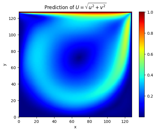
It can be seen that at \(Re=1000\), the prediction result is basically the same as the solver result (L2 relative error is 7.7%).

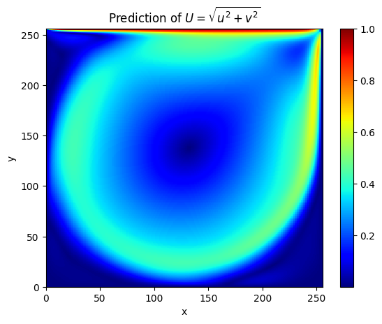
It can be seen that at \(Re=3200\), the prediction result is basically the same as the solver result (L2 relative error is 4.1%).

6. References

• PIRATENETS: PHYSICS-INFORMED DEEP LEARNING WITHRESIDUAL ADAPTIVE NETWORKS
• jaxpi LDC example